Math 918, Spring 2026: F-Singularities

Course Documents

Course Announcement

Syllabus

• Linquan Ma & Thomas Polstra's F-Singularities: A Commutative Algebra Approach; called [MP] in the daily update.
• Alessio Caminata & Alessandro de Stefani's Notes for course on F-singularities; called [CdS] in the daily update.
• An additional resource is Karl Schwede & Karen Smith's Singularities defined by the Frobenius map; however note that this book requires more knowledge of algebraic geometry than is covered by the prereqs of this course, so I will not be explicitly suggesting it as complementary reading (even though their order of topics matches ours most closely!).

Office Hours: Mon 1:30-2:30 and Thurs 12:30-1:30. Or stop by my office when my door is open.

on MONDAY 04/27: Office hours moved to AFTER the RTG seminar (i.e., 3:30-4:30) so that I can watch the Math in the City presentations. I will also be around my office all afternoon prior to the presentations, so feel free to stop by between noon-ish and 1:30pm as well

Homeworks

• Homework 1: [PDF] and [TeX] + [math-hw.sty] (style file needed to compile!)
  • Due on Friday Feb 6th at midnight. Submit on Gradescope.
  • [Solution] to HW1.
• Homework 2: [PDF] and [TeX] + [math-hw.sty] (style file needed to compile! same as last week)
  • Due on Friday Feb 20th at midnight. Submit on Gradescope.
• Homework 3: [PDF] and [TeX] + [math-hw.sty] (style file needed to compile! same as last week)
  • Due on Friday March 6th at midnight. Submit on Gradescope.
• Homework 4: [PDF] and [TeX] + [math-hw.sty] (style file needed to compile! same as last week)
  • Due on Friday March 28th at midnight (three weeks because of spring break!). Submit on Gradescope.
• Homework 5: [PDF] and [TeX] + [math-hw.sty] (style file needed to compile! same as last week)
  • Due on Saturday April 11th at midnight. Submit on Gradescope.
• Homework 6: [PDF] and [TeX] + [math-hw.sty] (style file needed to compile! same as last week)
  • Due on Friday May 1st at midnight (three weeks due to late release!). Submit on Gradescope.

In-Class Handouts

• 02/03 Worksheet: [Fedder's Criterion]
• 02/05 Cheatsheet: [Macaulay2 Cheatsheet]

HCC Info

You have access to the Holland Computing Center (HCC) for this class! To use these resources, you will need an account associated with HCC that is separate from your University of Nebraska account and credentials:

• If you need an HCC account: https://hcc.unl.edu/new-user-request and request the math918 group.
• If you already have an HCC account from a prior class or research, you can add the class group to your account or move your account to the math918 group: https://hcc.unl.edu/group-addchange-request.
  Note: Not actually required to add/change group! ANY access to HCC is good enough for us. But you're still welcome to join the class group if you e.g. want to keep class access separate from research access for some reason.

**You will need to activate your DUO two factor for your HCC account in order to use the resources. Without this you will not have access! This is different from the TrueYou DUO you use to log into other UNL services.**

Here is some other important info:

• For more useful links and notes for students taking a class using HCC resources, please see https://hcc.unl.edu/docs/faq/class_students.
• While using HCC resources for this class, be aware of HCC's class account guidelines and center's policies: https://hcc.unl.edu/hcc-policies.
• Pay special attention to the guidelines for class accounts since data is removed at the end of the semester: https://hcc.unl.edu/hcc-policies#class-groups

Daily Update

Use this table of contents list to jump to a specific day. Info for future classes is a tentative plan, and will be updated by the day after the class with what actually happened.

Jan 13

Basics & Notation: Day 1

Jan 15

Basics & Notation: Day 2

Jan 20

Completions and Proof of Kunz's theorem

Jan 22

Finishing proof of Kunz's theorem + starting F-splitting

Jan 27

Proof that F-splitting can equivalently be checked for some/any $e$; examples (including F-finite regular local rings); the statement of Fedder's criterion; viewing $\hom_S(F_*^eS,S)$ as a rank 1 free module for regular $S$.

Jan 29

A HW correction; fact about the generating $\Phi$ and ideal containments; more general statement of Fedder's criterion.

Feb 03

F-splitting localizes; the F-split locus is open; the completion of Fedder.

Feb 05

We learned some M2 basics (everything needed to do Fedder's criterion) and also learned how the HCC works.

Feb 10

Defined (eventual) splitting along elements and SFR. Proved that local + SFR implies domain, and that F-finite regular local rings are SFR.

Feb 12

Fedder examples; proof that if $R$ is SFR then so is $R_{\mf p}$.

Feb 17

Proof that if $R_{\mf p}$ is SFR for all $\mf p$, then $R$ is SFR; proved that all F-finite regular rings are SFR; stated that for SFR rings all module-finite extensions split and started proof.

Feb 24

Finishing up Ch 3 of [MP]: finishing the above proof; doing the "test element" criterion that reduces checking SFR-ness to checking eventual F-splitting along a single (well-chosen) $c$, + a reminder of the Jacobian criterion for smoothness and how to use it to choose a good $c$.

Feb 26

Solutions to exercises on computing which of four rings $R$ were SFR; starting local cohomology.

Mar 03

More local cohomology basic properties + an example. (Proofs under construction

Mar 05

More local cohomology basic properties + a proof of the local cohomology characterization of Cohen-Macaulayness + defining the Frobenius action (Proofs under construction)

Mar 10

Matlis duality, its application to local cohomology (called local duality), and proving that for a complete local regular ring, we can detect the dimension of a module by looking at which local cohomology module is the top non-vanishing one. We ended with a NON-example of an F-injective. Proofs under construction!

Mar 12

Saw how the non-example generalizes a little bit and saw how weak normality connects to the Frobenius action on $H^1$. We (vaguely) defined the word F-singularity. Ended by showing that SFR implies CM in the complete case, and proved/stated other facts that we'll be needed to extend from the complete case to the general case. (Notes complete!)

Mar 24

Put everything from Mar 12 together to see why ALL SFR rings (which for us are all F-finite) are CM. Then we'll define F-rational as our last class of F-singularities, and see how F-rational fits into our singularity picture.

Mar 26

F-injective behaves well under deformation; and using this to see an example of an F-injective ring that is not F-split.

Mar 31

Starting applications of F-singularities! Combinatorics application to magic squares (and some general facts about the Hilbert polynomial).

Apr 02

Reduction to char p: Hochster-Roberts theorem that a subring of a polynomial ring with a "contracted" sop is a CM ring, statements of generic freeness.

Apr 07

Wrapping up reduction to char p---Hochster's meta-theorem + a "style of result" and some examples when it is actually true. Start of F-finiteness: partial proof that F-finite rings are excellent, + the "almost" converse; F-finite rings are quotients of F-finite regular rings,

Apr 09

Saw (without proof) an example of a regular but non F-finite ring which fails many of our earlier properties of regular rins. Start of F-purity! Definion of pure, F-pure, + some basic statements.

Apr 14

Finished F-purity, including proving the injective hull criterion for checking purity, and saw that for F-finite rings, R is F-pure iff it is F-split. Defined tight& Frobenius closure.

Apr 16

Test elements (for tight closure), tight closure of graded ideals, and a bunch of examples
Under construction!

Apr 21

Frobenius closure commutes with localization; tight closure does NOT commute with localization. Defined F-regular and weakly F-regular; saw how closure operations (tight/Frobenius on all/parameter ideals) relate to the four F-singularities. In some cases we got an exact characetrization; in some cases only one direction.

Apr 23

Wrapped up tight closure: colon capturing, persistence, the char p version of Hochster-Roberts, and big balanced CM algebras. Stated Peskine-Szpiro vanishing (finite pd implies Tor's against $F_*^eR$ vanish) and proved the acyclicity lemma.
Still under construciton!

Apr 28

Finished proof of Peskine-Szpiro vanishing, and the corollary that the PS functors are exact on the category of modules of finite pd (so, a more general version of the direction of Kunz's theorem that regular implies PS functors are exact).
Still under construction!

Apr 30

Clarified the module action that comes from applying the Peskine-Szpiro functors. Stated Herzog's converse to PS's theorem; some effective bounds from Koh+Lee (i.e., when a finite number of Tor vanishings suffice to prove that $M$ has finite pd). Also saw more ways of using the Frobenius to detect regularity. Specifically, Rodicio's theorem and Avramov+Iyengar+Miller's theorem on how finite flat/injective dimension of $F_*^eR$ implies $R$ is regular.
20 minute speed run of "what is a scheme" up thru the geometric notion of global Frobenius splitting; some warnings of how similar looking vocab is used in AG papers to maen related (but slightly different!) things than in CA papers. Finally, some open questions.

Jan 13

Big Assumptions (for all semester!): p = a prime number; q = a power of p; all rings are unital, commutative, and noetherian. For a very long time (up until reduction to char p), all rings are characteristic p.

We covered the beginning of Ch 1 of [CdS], up through and including Remark 1.8. (See also very first section of [MP].) Useful fact: In a reduced (char p) ring, when p-th roots exist, they are unique!

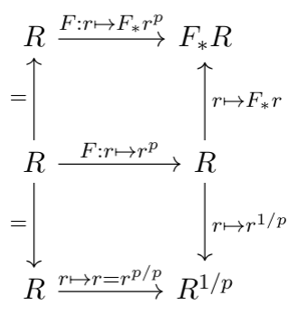
We also concretely looked at $R^{1/p}$ and $F_*R$ in the concrete example where $R=\mathbb F_2[x]$, and saw how these are generated (as $R$-modules) by $\{1,\sqrt x\}$ and $\{1,F_*x\}$, respectively. We saw more generally that when $R= \mathbb F_p[x_1,\ldots, x_n]$, that $F_*R$ is generated by $\{F_*(x_1^{a_1}\cdots x_d^{a_d})\: | \: 0\leq a_i \lt p\}$. We even saw that this generating set is actually a basis! Finally, the following commutative diagram showed us that all three perspectives are really "the same" map. Note that all vertical maps are isomorphisms/equalities, the horizontal maps are all different ways of writing the Frobenius, and the whole bottom row only makes sense when $R$ is reduced.

Jan 15

Defined a separable polynomial and a perfect field (Ref: Section 15.5 of Eloísa's Math 818 notes). In particular, a char $p$ field is perfect if and only if $F$ is a surjection. $K=\mathbb F_p(T)$ is a non-perfect field example. We stated #5 below as a bonus problem (but originally stated it wrong! I meant to say $R^p$ not $R^{1/p}$, my apologies).

We then worked for a while on questions #1-4, and went over the answers to #1-3:

1. Describe the $R$-module structure of $F_*R$ when $R=\mathbb F_p[x,y]/\langle xy\rangle$. View Solution

   Generators are $\{F_*x^i, F_*y^i\: | \: 0\le i \lt p\}$. I.e., the same as for the polynomial ring, but we remove all the ones corresponding to the cross terms that are already zero in this quotient ring.

   Relations are $yF_*x^i = 0$ and $xF_*y^i=0$.

2. Describe the $R$-module structure of $F_*R$ when $R=\mathbb F_2[x^2,x^3]\subset \mathbb F_2[x]$. View Solution

   Generators are $\{F_*1, F_*x^2, F_*x^3, F_*x^5\}$. Notice that the monomials in $R$ are every power of $x$ EXCEPT for $x$ itself. So via taking $x^aF_*x^b = F_*x^{2a+b}$ for $b\in \{0,2,3,5\}$, we see that even just $F_*x^{2a+2}$ and $F_*x^{2a+3}$ cover all possible powers $\ge 6$. The only other seemingly missing monomial is $F_*x^4$, but $F_*x^4 = x^2F_*1$.

   Relations are   $\begin{aligned} x^3F_*1 &= x^2 F_*x^2 & x^3F_*x^3 &= x^2F_*x^5 \\ x^4F_*1 &= x^3F_*x^2 & x^4F_*x^3 &= x^3F_*x^5\end{aligned}$.

3. Describe the $R$-module structure of $F_*R$ when $R=\mathbb F_3[x,y]/\langle y^2-x^3-x\rangle$. View Solution

   Generators are $\{F_*1,F_*x,F_*y\}$. Clearly the 9 monomials $\{F_*x^iy^j\: | \: 0\le i,j\lt 3\}$ would suffice as a generating set, so now we'll show that the other 6 of them are actually redundant via taking multiples of our defining equation. As we go down the list, we will only use higher up monomials to get the lower ones.

   • $F_*y^2 = xF_*1 + F_*x$ (via original equation)
   • $F_*xy = yF_*1 - xF_*y$ (via $\cdot y$)
   • $F_*xy^2 = yF_*y - xF_*y^2$ (via $\cdot y^2$)
   • $F_*x^2 = F_*xy^2 - xF_*x$ (via $\cdot x$)
   • $F_*x^2y^2 = xF_*x^2 + xF_*1$ (via $\cdot x^2$)
   • $F_*x^2y = yF_*x - xF_*xy$ (via $\cdot xy$)

   There are no relations!

4. Describe the $R$-module structure of $F_*R$ when $R=\mathbb F_p(T)[x]$. View Solution

   Generators are $\{F_*(T^jx^i)\: | \: 0\le i,j\lt p\}$. No relations!

   Notice that $TF_*x^i = F_*(T^px^i)$. So if we had only used the generators from the perfect field case, we would be missing being able to write an element like $F_*T$. Or said another way, previously in the perfect case we knew that if we wanted to write $F_*(ax)$, we could always pull out the $a$ via taking a $p$-th root, so that $F_*(ax) = a^{1/p}F_*x$. But if the Frobenius isn't surjective, we can't do that anymore!

5. Give an example of a ring $R$ where $R^{p}$ is NOT isomorphic to $F_*R$. In other words, an example where the inclusion $R^p\hookrightarrow R$ is NOT the same map as the Frobenius. [Corrected typo from earlier statement: I wanted $R^p$ not $R^{1/p}$!]

We then noticed a pattern: drawing the corresponding varieties for the two ``free'' examples gave us affine space (the polynomial ring) and a smooth elliptic curve (#3). Drawing the two ``non-free'' examples gave us two lines crossing (#1) and a cuspidal cubic (#2).

You will eventually learn a lot more about regular rings in Math 906.

For a local ring and a finitely generated module $M$, you already know that $M$ is flat if and only if it is free. This and our new definition give us an immediate corollary to Kunz.

Jan 20

Some facts (that became exercises):

1. Prove that $F$ induces an isomorphism on Spec. View Solution

   The induced map on Spec takes a prime ideal $Q$ to $F^{-1}(Q)$. If $r\in Q$, then $r^p=F(r)\in Q$ and thus $r\in F^{-1}(Q)$. Conversely, if $r\in F^{-1}(Q)$ this means $r^p\in Q$, but $Q$ is prime so $r\in Q$.

2. Prove that $F_*^e$ is an exact functor. (In particular, we first saw what it does to maps and to modules: just throws an $F_*^e$ decoration in front!) View Solution

   See proof of Prop 1.10(1) in [CdS].

3. If $W\subset R$ is a multiplicative set, then $W^{-1}(F_*^eR)\to F_*^e(W^{-1}R)$ via $\frac{F_*^e r}{w}\mapsto F_*^e(\frac{r}{w^{p^e}})$ is a $W^{-1}R$-module isomorphism. View Solution

   See proof of Prop 1.10(2) in [CdS].

Proof of Kunz's theorem (regular implies flat):

$R$ is regular iff $R_Q$ is regular for all $Q$; and a map $\phi$ is flat iff $\phi_Q$ is flat for all $Q$. Further, $F_*^e$ commutes with localization. Thus we reduce to the local case. Now consider

Recall fact: In such a diagram (where both vertical maps are faithfully flat), if the bottom map is flat then so is the top one. So sufficient to show for the complete case, and likewise sufficient to do for a power series ring over an algebraically closed field, but we (basically) already did that!  ■

We started the proof of the other direction (in the style of [CdS]) but didn't finish; however we did get through the following:

Proof in Lemma 2.6 of [CdS]

Jan 22

Proof: Let $I=\underline x$. Then by Lech independence, $I/I^2 \cong (R/I)^n$ as $(R/I)$ and as $R$-modules. But then flatness gives \[ (IS)/(IS)^2 \cong (S/IS)^n \] and by rank reasons clearly $\varphi(\underline x)$ is still a minimal generating set.  ■

Proof: From last time, we saw that $\underline x : y_1 = \langle z_1,x_2,\ldots, x_n\rangle$. So suppose we have coefficients $a_1z_1 + \sum_{i=2}^n a_ix_i=0$. Multiply by $y_1$ to get $a_1(y_1z_1)+\sum_i (a_iy_1)x_i=0$. By Lech independence of $\underline x$, this means $a_1 \in \underline x \subset \langle z_1,x_2,\ldots, x_n\rangle$. Further, means $a_i \in \underline x:y_1 = \langle z_1,x_2,\ldots, x_n\rangle$ as desired.  ■

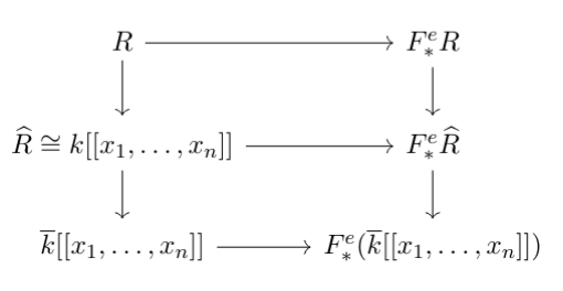
Proof of Kunz's theorem (flat => regular): $R$ is regular if and only if $\widehat R$ is regular, and by the same diagram before, if $F_*\widehat R$ is a flat $\widehat R$ module then $F_*R$ is a flat $R$-module. (In fact, this is iff because $\widehat R\to \widehat{F_*R}$ is canonically $\widehat R\to F_* \widehat R$.) So WLOG $R$ is complete local ring, and $R\cong k[[x_1,\ldots, x_n]]/I$. Let $S=k[[x_1,\ldots, x_n]]$.

We can further WLOG assume $n =$ embedding dimension (recall that = $\dim_k\mathfrak m / \mathfrak m^2$ = by NAK the minimal number of generators of $\mathfrak m$), since if not just throw away redundant $x$'s. Thus $\underline x$ is Lech independent, and so is $\underline x^{[q]}$, and then also so is $x_1^{a_1},\ldots, x_n^{a_n}$ for combo of powers.. On the one hand, by Lech's length lemma, a base case of $\ell(R/\mathfrak m)=1$, and induction, we get that $\ell_R(R/\langle x_1^{a_1},\ldots, x_n^{a_n}) = \prod_i a_i$. But we also can do the same thing to $S$ and see that $\ell_S(S/\langle x_1^{a_1},\ldots, x_n^{a_n}) = \prod_i a_i$.

Thus $S/\langle \underline x\rangle^{[p^e]}\to S/(I+\langle \underline x\rangle^{[p^e]}\cong R/\mathfrak m^{[p^e]}$ is an isomorphism for all $t$, and so $I\subset \underline x^{[q]}$ and by Krull's intersection, $I=0$.   ■

Now... new topic! Moving onto Frobenius splitting. We defined F-splitting, saw a proposition about how it relates to other split maps, and saw two examples.

We saw that was the same since being a splitting exactly means that for all $r\in R$ we have $r = \pi\circ F(r) = \pi(F_*r^{p})=\pi(rF_*1)=r\pi(F_*1)$.

Proof: Let $\pi:F_*R\to R$ be our splitting. If $\pi\circ F=\operatorname{id}_R$, this forces the first map to be injective. And we saw $F$ injective iff $R$ reduced.  ■

Proof: Suppose that $\varphi$ is split via $\gamma:S\to R$, and that $F_S$ is split via $\pi:F_*S\to S$. Then $\gamma\circ\pi\circ (F_*\varphi)$ is our desired splitting of $F_R$. See this via \[\gamma\circ\pi\circ (F_*\varphi)(F_*1) = \gamma\circ \pi(F_*\varphi(1)) = \gamma(\pi(F_*1))=\gamma(1)=1.\quad ■\]

Today's class prompted some good requests for examples, which I will give you on Tuesday:

• What's an example of a reduced ring that is NOT F-split?
• What's an example of an invariant ring that is F-split even though $p||G|$?

Finally, an in-class exercise was to prove the following, which we will go over on Tuesday:

Jan 27

Proof of Proposition 4.8 from last week (F-split iff for some e iff for all e): 1 implies 3: If $\pi:F_*R\to R$ is our splitting, then notice that $\pi\circ F_*\pi \circ \cdots \circ F_*^{e-1}\pi:F_*^eR\to R$ is a splitting! Notation $\pi^{\star e} =$ such a composition, and in fact $\psi\star \phi := \psi\circ F_*^e\phi$.

3 implies 2: clear

2 implies 1: let $\pi:F_*^eR\to R$ be our splitting. Then \[ R \stackrel{F}{\to} F_*R \stackrel{F_*F^{e-1}}{\to} F_*^eR \stackrel{\pi}{\to} R \] so take $\pi \circ F_*F^{e-1}$ as our splitting.   ■

(Non)Example 5.1: The ring $\mathbb F_2[x^2,x^3]$ is reduced, but is NOT F-split. (Proved in HW 1 #4).

Example 5.2: Here are some invariant rings that ARE F-split even though $p$ divides the order of the group (so that the Reynold's operator proof won't work):

• If $G$ acts via the trivial action, then for ANY ring $R$ we have $R^G=R$. So regardless of the group order, if $R$ is F-split then clearly so is $R^G$.
• If $G=S_2$ and $R=\mathbb F_2[x,y]$ and we do the same symmetric group action of permutating the variables from last time. Then $R^G = \mathbb F_2[x+y,xy]\cong \mathbb F_2[w,z]$ which is regular and thus F-split.

The following theorem was an in-class exercise.

WARNING: It is NOT true that every regular local ring is F-split; we really do need some adjectives! We will see an example later in the semester.

It's stated there for motivation but it will take us a while to prove it. First we want to have a good understanding of what $\hom_S(F_*^eS,S)$ looks like, and how it relates to $\hom_R(F_*^eR,R)$. This will then help us figure out how a potential splitting of the Frobenius on $R$ might relate to one on $S$.

Proof (when $k$ is perfect): $k$ is perfect means we don't have to worry about the $\lambda_i$ (a similar proof works with them there it is just more annoying to type out but not any more interesting). Let $\pi_\alpha$ be the dual (projection) to $x^{\alpha}$, so that \[ \pi_\alpha(F_*^e(x^{\beta})) = \begin{cases} 1 & \alpha = \beta\\ 0 & \textrm{else} \end{cases}. \]

• Goal 1: Show that each $\pi_\alpha$ can be written as $F_*^es\cdot \Phi$ for some $s\in S$. (Hint: First notice that $\Phi$ itself is a $\pi_\alpha$, and then see what $F_*^ex\cdot \Phi$ looks like in terms of the $\pi_\alpha$'s, and see if you can figure out a pattern.) View Goal 1 Proof

  Let 𝟙 denote the all 1's vector. So $\Phi = \pi_{(p^e-1)𝟙}$, and more generally we HAVE a map that sends exactly one monomial to 1 (and the rest to 0), and we WANT maps that send exactly one monomial to 1 (and the rest to 0). So we should try acting by monomials. Specifically, \[F_*^e(x^{(p^e-1)𝟙-\alpha})\cdot \Phi (F_*^ex^{\beta}) = \Phi(F_*^e x^{(p^e -1)𝟙-\alpha+\beta}) = \begin{cases} 1 & (p^e-1)𝟙 - \alpha+\beta = (p^e-1) 𝟙 \\ 0 & \textrm{else}\end{cases}.\] I.e., it equals one exactly when $\beta = \alpha$. So $F_*^e(x^{p^e𝟙 -1 -\alpha})\cdot \Phi = \pi_\alpha$.   ■

  Observation: This shows why we needed $\Phi$ to send the LARGEST generator to zero. Otherwise the $x^{ (p^e-1)𝟙 -\alpha}$ we are acting by would have had the $(p^e-1)𝟙$ replaced by something smaller, and so the whole exponent would have been negative sometimes (bad because we're in a polynomial/power series ring).

• Goal 2: Show that the $\pi_\alpha$ generate $\hom_S(F_*^eS,S)$ as an $F_*^eS$ algebra. View Goal 2 Proof

  Consider a map $\psi:F_*^eS\to S$. If we build a map that agrees with $\psi$ on the generators $x^\alpha$ then we're done. So define our candidate map \[\varphi= \sum_\alpha F_*^e(\psi(x^\alpha))^{p^e} \cdot \pi_\alpha \] which ensures \[\varphi(F_*^e(x^\beta)) = \sum_\alpha( F_*^e(\psi(x^\alpha)^{p^e}) \cdot \pi_\alpha)(F_*^ex^\beta) = \sum_\alpha \pi_\alpha(F_*^e(\psi(x^\alpha)^{p^e}x^\beta)) = \sum_\alpha \psi(x^\alpha)\pi_\alpha(F_*^ex^\beta) = \psi(x^\alpha)\pi_\alpha(F_*^ex^\alpha) = \psi(x^\alpha)\] as desired. Notice the magic that happened here---our action only allows us to act via pre-multiplication. However, by acting by a $p^e$-th power of an element, we get the same answer as if we acted by post-multiplication! In other words, the usual fact that the $\pi_\alpha$ generate as an $S$-basis (by typical dual basis fact) is also why we're getting that these generate over $F_*^eS$.   ■

Now clearly combining Goal 1 and Goal 2 we see that $\Phi$ generates. For freeness, the only possible relation is of the form $F_*^es \cdot \Phi=0$. But this can never happen---$\Phi$ is non-zero on monomials of arbitrarily large degree!   ■

Jan 29

Proof: If $J\subset I^{[p^e]}$, then in fact for ANY map $\psi\in \hom_S(F_*^eS,S)$ we have \[ \psi(F_*^eJ)\subset \psi(F_*^eI^{[p^e]}) \subset I\psi(F_*^eS)\subset I. \] For converse, first make several observations: By Kunz $F_*^eS$ is free over $S$, with basis $\{F_*^eg_i\}_{i=1}^t$. Let $\{\pi_i\}_{i=1}^t\subset \hom_S(F_*^eS,S)$ be the dual basis (recall: this means $\pi_i(F_*^eg_j)=1$ if $i=j$, otherwise $0$). Further, because $\Phi$ generates, there exist $s_i\in S$ s.t. $\pi_i = F_*^es_i \cdot \Phi$. And \[\id_{F_*^eS} = \sum_i \gamma_i \circ \pi_i,\] where here $\gamma_i$ is the $S$-module map $S\to F_*^eS$ which sends $1\mapsto F_*^eg_i$. (Notice: this is the same as taking the $e$-th Frobenius map $S\to F_*^eS$, and then composing with multiplication by $F_*^eg_i$).

Now since $\Phi(F_*^eJ)\subseteq I$, we see \[\pi_i(F_*^eJ) = (F_*^es_i \cdot \Phi)(F_*^eJ) =\Phi(F_*^e(s_iJ))\subseteq I\] and so further, \[ F_*^eJ = \id_{F_*^eS}(F_*^eJ) = \sum_i \gamma_i \circ \pi_i(F_*^eJ) \subseteq \sum_i \gamma_i(I) = \sum_i I\gamma_i(S)\subseteq I \] as desired.   ■

Proof: The natural map: Let $t\in I^{[p^e]}:I$ and $\varphi\in \hom_S(F_*^eS,S)$. Given $r+I\in S/I=R$, we ideally want the resulting map on $\hom_R(F_*^eR,R)$ to have $F_*^e(r+I)\mapsto (F_*^et\cdot \varphi)(F_*^er) + I$. This will work! To check it is in $\hom_R(F_*^eR,R)$ we only need to check well-definedness, i.e., that things in $F_*^eI$ are sent to things in $I$. Sosuppose we have some $j\in I$. Then \[(F_*^et\cdot \varphi)(F_*^ej) = \varphi(F_*^e(jt))\in \varphi(F_*^e(I^{[p^e]}) = I\varphi(F_*^eS) \subset I.\] And by design, the overall map $\Psi$ is an $F_*^eS$-module map.

Surjectivity in the regular case: Since $S$ is regular we have $F_*^eS$ flat (by Kunz). Since $S$ also F-finite, we further have $F_*^eS$ a projective $S$-module. Thus ANY map $\theta\in \hom_R(F_*^eR,R)$ can be lifted to $\Theta\in\hom_S(F_*^eS,S)$ (using that the projection map $\rho:S\to R$ is surjective). By our knowledge of $\hom_S(F_*^eS,S)$, we can write $\Theta = F_*^es \cdot \Phi$. To finish surjectivity, it will suffice to check that $s\in I^{[p^e]}:I$. But by virtue of the fact that $\Theta$ descends, \[I\supset \Theta(F_*^eI) = \Phi(F_*^e(sI)).\] Now by the Proposition above, $sI\subset I^{[p^e]}$, thus $s\in I^{[p^e]}:I$.

Kernel in the regular case: A map $F_*^et\cdot \varphi\in F_*^e(I^{[p^e]}:I)\cdot \hom_S(F_*^eS,S)$ is in the kernel if it descends to the zero map, which happens exactly when $(F_*^et\cdot \varphi)(F_*^eS) = \varphi(F_*^e(tS))\subset I$. Now use the Proposition again, further writing $\varphi = F_*^es\cdot \Phi$, so that $\Phi(F_*^e(stS))\subset I$ and so $stS \subset I^{[p^e]}$. Thus $st\in I^{[p^e]}$, and we've shown that $F_*^et\cdot \varphi = F_*^e(st)\cdot \Phi$ is in $F_*^e(I^{[p^e]})\cdot \hom_S(F_*^eS,S)$ as desired.   ■

The following theorem has been restated for clarity. (It was still true as stated in class though!)

Proof is promised for February 3rd!

Proof of Fedder's criterion ($I^{[p^e]}:I\not\subseteq \mf m$ version from Jan 27) using the above: Let $(R,\mf m)$ be our local ring. By the Lemma from Feb 3rd, $R$ is F-split if and only if $R_{\mf m}$ is F-split, i.e., $R$ is F-split at $\mf m$. By the above Theorem, this is if and only $(I^{[p]}:I)\not\subseteq \mf m^{[p]}$, as desired.   ■

Feb 3rd

Today had a worksheet: [Fedder's Criterion]

Finishing the proof of the (more general) Fedder's criterion, including some necessary lemmas. Hopefully some examples. Also, set up an HCC account by Thursday if you want to follow along with the demo!

The following results will appear as exercises, in addition to a few more examples (squarefree monomial ideals?)

The arguments for (1) iff (3) and for (1) iff (4) follow similarly.  ■

Remark 7.7: The ``locus'' of F-split points is the set of points $\mf p$ on which $R$ is F-split. On Spec, points are prime ideals, and "being F-split at prime ideal $\mf p$ means that $R_{\mf p}$ is F-split. Finally, open means in the Zariski topology, where all open sets look like $U=\Spec R\setminus \bb V(J)$ for an ideal $J$.

Putting this all together... By the Theorem 6.3 on hom structure from Jan 29 (and by the fact that $I^{[p^e]}:I$ is an ideal), EVERY map in $\hom_R(F_*^eR,R)$ comes from a map of the form of Lemma 7.3. (See this because for any $t'\in I^{[p^e]}:I$ and $\gamma\in \hom_S(F_*^eS,S)$, we can write $\gamma = F_*^es \cdot \Phi$, and so $F_*^e(t')\cdot \gamma = F_*^e(t's)\cdot \Phi$. )

By Lemma 7.1, there exists a $\varphi$ which is surjective when descended to $R$ iff $R$ is F-split. By Lemma 7.3, this happens iff there exists a $t\in I^{[p^e]}:I$ which is $\notin \mf m^{[p^e]}$. In other words, iff $I^{[p^e]}:I\not\subset \mf m^{[p^e]}$. This (FINALLY!) completes the proof of Fedder's criterion, and in fact in a stronger way where we see we could've done some/any $e$ instead of just $e=1$.   ■

Feb 5th

Today had a handout: [Macaulay2 Cheatsheet]

Macaulay2 (M2) related links

• Web Macaulay2: https://www.unimelb-macaulay2.cloud.edu.au/
• The Macauly2 Documentation: https://macaulay2.com/doc/Macaulay2/share/doc/Macaulay2/Macaulay2Doc/html/
• The M2 Zulip chat (Zulip is a chatroom kinda like slack or discord; this can be a useful place to go with code questions): https://macaulay2.zulipchat.com/
• The M2 GitHub (not needed for most people, but could be useful if you want to install on your personal laptop, or if you want to file a bug report or contribute to code!): https://github.com/Macaulay2/M2
• Advanced users: You can pass command-line arguments to a .m2 file run as a script using scriptCommandLine and value in your M2 code.

Holland Computing Cluster (HCC) related links

• Swan Open OnDemand (aka, the way to access the HCC through a browser): https://swan-ood.unl.edu/ . You know you set up your account correctly if you are able to login at that link!
• HCC documentation: https://hcc.unl.edu/docs/
• Guide to basic shell (aka terminal aka console) commands: https://hcc.unl.edu/docs/connecting/basic_linux_commands
• VERY advanced users: You can pass in command line arguments to an sbatch command via the instructions in this stackexchange post.

Running M2 on HCC in interactive mode

To run Macaulay2 on the HCC in interactive mode... First go to Swan Open OnDemand. Click the dropdown menu for "Clusters" (in the red bar on top), then click the only option which is Swan Shell Access. You're now in a black background, text-only shell! Then run the following three commands one-by-one (commands themselves in the numbered list, comments/context bulleted in underneath each):

1. srun --pty --mem=10gb --qos=short $SHELL
   • Before running this line, the "prompt" (place I'm typing) looks something like
     [username@login1.swan ~]$
   • This command might take a minute or two to run, with messages saying something about being queued, waiting for resources, and/or having resources allocated. Once it has completed, your new prompt will look something like
     [username@c0000.swan ~]$
   • What's going on here?
     srun
     = "slurm run", i.e., running a "real time" job using SLURM (what SLURM is doesn't matter, but it does mean a lot of commands start with s...).
     pty
     = a specific interface format.
     mem
     = an amount of memory. I wouldn't ever go less than 10gb even for a "small" job because even just opening M2 can take some space!
     qos
     = "quality of service", aka how the system decides priority (if more people want to run code RIGHT NOW than the system can handle, who gets to go first?). So short means we'll get cut off after 6 hrs, and it might be sooner if tons of people are also requesting short jobs.
2. module load apptainer
   • By default installed programs aren't actually accessible to you, you need to "module load" them first. For example, "module load python". Here, "apptainer" is a way to get weirder and more niche programs.
3. apptainer exec docker://unlhcc/macaulay2 M2
   • This starts up M2, including "installing" it. The first time you do it, it might take a while (for me it took under 10 minutes, but more than 5). However, it will cache the result in something called a SIF file to make future loads faster! So if you ever see output messages about using cached SIF files, that's usually a good thing :)

TADA! After this you should now be in M2 interactive mode.

Uploading Files to HCC

Easy way:

1. Go to Swan Open OnDemand.
2. Click the dropdown menu for "Files" (in the red bar on top), then select "Work (math918)". Note: You can also use the "Home Directory" button, however, code run from Work will be faster!
3. The page now shows a list of files (or maybe is empty if it's your first time). In the upper right, there are some white and blue buttons. Use the blue Upload button to upload a new file (for example, the demo files from below).Or use "New File" to create a new file from scratch (for example, to copy paste some M2 code from the web version).

From this screen you can also create/edit files! The New File button is near the upload button, and is useful for copy-pasting M2 code from the web version. To edit an existing file, scroll down to it in the list and click the meatball menu (3 vertical dots). Both of these (new file or edit) open a file editor. Be sure to save in the upper left when done!

Harder way: Use the scp (secure copy not slurm copy). From your laptops terminal, type
scp /path/to/laptop/file username@swan.unl.edu:/work/math918/username

Submitting an asynchronous M2 job to the HCC (aka submitting a batch script)

The files from class: [Sample Batch Script] + [demo.m2]. Upload using instructions above!

To submit this, first need to get into the Swan Shell again. Login to Swan Open OnDemand. Click the dropdown menu for "Clusters" (in the red bar on top), then click the only option which is Swan Shell Access. You're now in a black background, text-only shell!

Now we need to find where the .submit file is. Here are several useful commands:

• ls
  LiSts what is in the current directory. (Do the files look like what you expected to see?)
• pwd
  Prints Working Directory, i.e., tells you the name of the folder you're currently in.
• cd /path/to/new/directory
  Changes Directory to wherever you said. Useful special cases on the HCC are
  cd /work/math918/username   or   cd $WORK   to go to your work directory;
  cd /home/math918/username   or   cd $HOME   to go to your home directory;
  cd ..   (yes that's two periods no spaces in between them as the path to the file!) to go up one directory level.

Use that to get yourself to the directory with the .submit file. (If you followed the instructions under uploading, all you should need to do is cd $WORK   but it is recommended to use ls   to double check. Finally, run the following command:

where sbatch = "slurm batch", and you can replace helloworld.submit by any batch file.

Modifying helloworld.submit: To run an ACTUALY M2 file you care about, just change demo.m2 to the filename you actually want. For more advanced things, here's what's going on inside this file:

• Line 1 says "#!/bin/bash". Don't touch this!
• Look at the 2nd & 3rd lines, about runtime and memory. Do you need to request longer? Shorter? More memory? Less memory? If your job uses more time/space than requested the HCC will shut it down :( On the flip side, requesting execessive space/time will take it longer to get scheduled, and since the HCC is a shared resource, is rude.
• Line 4 is how the job name will appear in the queue. Only matters insofar as it is helpful to you, you can name every single job helloworld if you want.
• Lines 5 & 6 say where to put the output & any error messages. If the name starts with a number or letter (just plain helloworld.%J.err) then it will save the file in the same directory you're in when you run sbatch. If the name starts with a slash (like /work/math918/abrosowsky/helloworld.%J.err) then it will put it in that specific folder, even if you're running sbatch from home instead of work.
  If using the version from in class, DEFINITELY change abrosowsky to be your username otherwise you won't be able to access any of the output files. As of 02/09 evening I've changed the format so that my username no longer appears.
• Replace demo.m2 in the last line of the file with the name of the m2 file you care about. Also, delete any echoes you want that's just for debugging demo purposes. There are only two lines that actually matter (not counting the # ones):
  module load apptainer
  apptainer exec docker://unlhcc/macaulay2 M2 --script demo.m2

Possible alternate method: The nice people at the HCC have made us a job template! In Swan Open OnDemand, click the dropdown menu for "Jobs" (in the red bar on top), then click "Job Composer". The macaulay2 template is called Apptainer-macaulay2-job. I still haven't figured out how to actually use the job composer but this might be helpful!

Troubleshooting

Error Messages? Take a look at the .err file. Does it give anything useful? My rule of thumb: totaly mysterious error usually = ran out of memory

Missing files? Did your output end up in home or in work? In a subfolder? Do you have two different HCC groups and put it in your advisor's group instead of the math918 group? Look through different options in the file browser, and double check in the batch file where you told it to save.

Other problem? Do you have another problem I should add to this list? Let me know!

Feb 10

F-splitting is nice, but can we do better? Our goal: describe a stronger condition on the ring that is still related to the Frobenius, but gets us even nicer properties.

Proof: See Tuesday 02/03! Same statement just new vocab.   ■

Proof: If $R$ is $e$-F-split along $c$, then since $1|c$ we have that $R$ is $e$-F-split along 1. By definition this means there exists a $\varphi$ such that $\varphi(F_*^e1)=1$.  ■

Proof: Suppose $\varphi$ is our $e$-F-splitting. By the Corollary, we also know that $R$ is F-split, and so let $\pi\in \hom_R(F_*R,R)$ be our Frobenius splitting. Then $\pi\circ F_*\varphi$ is our desired map, since $$\pi\circ F_*\varphi (F_*^{e+1}c) = \pi(F_*\varphi(F_*^ec)) = \pi(F_*1) = 1  ■ $$

Proof Method 1: (contrapositive) Suppose $cy=0$ for $y\neq 0$. Then our map that we are trying to split sends $y\mapsto F_*^ey^{p^e}\mapsto F_*^e(y^{p^e}c) = F_*^e0$. So the map isn't injective and can't be split.   ■

Proof Method 2: (contradiction) If we did have a splitting $\varphi$, we would have $$y = y\varphi(F_*^ec) = \varphi(F_*^e(y^{p^e}c)) = \varphi(F_*^e0) = 0$$ which is our desired contradiction.   ■

Proof that equiv (2) and original are the same definition: Recall that the set of zerodivisors is the union of all the elements in the associated primes, and that minimal primes are always associated. So if $R$ satisfies (2), then it automatically satisfies the original (since if you are a non-zero divisor you are DEFINITELY not in any minimal prime).

Conversely suppose that $R$ satisfies the original. Since 1 is a non-zero divisor, $R$ is eventually F-split along $1$, i.e., $R$ is plain old F-split. Thus $R$ is reduced, and reduced rings have no non-minimal associated primes.   ■

We had some good discussions about F-finiteness, and I'm going to summarize it here: I'm following the convention of the books we're using, and making F-finite part of the definition of SFR. This means that saying it in the previous theorem statement is redundant! I'm going to do that a lot though for emphasis.

As Adam pointed out in the chat, the original definition of strong F-regularity did not require F-finiteness, and indeed there's nothing in the definition that needs it there. In particular while all of our references require this, it's not always required out in the wild. For more about F-singularities in the non-F-finite world, check out these notes by Takumi Murayama.

Fact 9.11: (we won't prove this) There exists a char $p$ ring $R$ which is regular, but such that $\hom_R(F_*R,R)=0$. In particular, this is a regular ring which is neither SFR nor even F-split.

Proof: We only prove $n=2$, the rest is straightforward induction. If $\mf p_1\subset \mf q$, we're done. Otherwise there exists $a\in \mf p_1\setminus \mf q$. Observe that $\mf p_1\mf p_2\subset \mf p_1\cap \mf p_2$. For all $b\in \mf p_2$, $ab\in \mf q$ which by primeness means $b\in \mf q$ as desired.   ■

Proof omitted

Proof: The forward implication is clear. For the backgwards implication, let $\psi = F_*^e(\frac{1}{u^{p^e}})\cdot \varphi$. Then $\psi(F_*^ec) = \varphi(F_*^e(\frac{c}{u^{p^e}})) = \frac{1}{u}\varphi(F_*^ec) = \frac{1}{u}u = 1$.   ■

Proof of SFR + local implies domain: See proof of Lemma 3.2 in [MP].   ■

Proof: See proof of Theorem 3.4 in [MP] (ignoring the 1st line about reducing to the local case because we, by assumption, are already in the local case!)   ■

Feb 12

We started with a return to Fedder's criterion.

1. Let $k$ be an F-finite field and let $S=k[x_1,\ldots, x_d]$ be a polynomial ring. Let $I$ be a squarefree monomial ideal (so, $I=\langle m_1,\ldots, m_t\rangle$ where each $m_i$ is a monomial with no power $\gt 1$ on any variable). Prove that $S/I$ is F-split. View Solution

   Let $g=(x_1\cdots x_d)^{p-1}$. Then $m_i^{p-1}|g$, and so $m_i^p|(m_ig)$, and so $g\in I^{[p]}:I$. But clearly $g\notin \mf m^{[p]}=\langle x_1^p,\ldots, x_d^p\rangle$, thus $S/I$ is F-split as desired.

2. Let $k$ be an F-finite field and let $S=k[x,y,z]$. Let $f=x^3+y^3+z^3$. For which $p$ is $S/f$ F-split? View Solution

   We know that $\langle f\rangle ^{[p]}:\langle f \rangle = \langle f^{p-1}\rangle$. Exapanding out, $$f^{p-1} = \sum_{a+b+c=p-1} \binom{p-1}{a,b,c} x^{3a}y^{3b}z^{3c}.$$ If one of these monomials is NOT in $\mf m^{[p]}$, we need $3a,3b,3c\lt p$, i.e., we need $a,b,c,\le \lfloor \frac{p-1}{3}\rfloor$. On the flip side, since $a+b+c=p-1$, this means we need $3\lfloor \frac{p-1}{3}\rfloor \geq p-1$, i.e., $\lfloor\frac{p-1}{3}\rfloor\geq \frac{p-1}{3}$. But a floor usually makes things smaller so this is only achieved when we have equality and $3|(p-1)$, i.e., when $p\equiv 1\mod 3$. Finally, note that the coefficient of $\binom{p-1}{a,b,c}$ is never $0$ mod $p$, since the numerator of $(p-1)!$ is never divisible by $p$.

Remark 10.1: A Stanley-Reisner ring is a polynomial ring mod a squarefree monomial ideal. Thus you have just proven that Stanley-Reisner rings are always F-split.

With those facts, we could compute $I^{[p]}:I$ in the Stanley-Reisner case if we wanted to... but it would be kind of annoying so our method is better! Check out the Wikipedia page on colon ideals for various other helpful properties of colon ideals.

Proof that SFR implies localizations are SFR: (Ref: Lemma 3.3 of [MP]) Suppose $R$ is strongly F-regular and let $\Min(R) = \{P_1,\ldots, P_n\}$, and let $\{P_t,\ldots, P_n\}$ be the primes of $R$ corresponding to the minimal primes of $R_{\mf p}$. Let $c\in R$ be such that $c/1 \in R_{\mf p}$ isn't contained in any minimal primes of $R_{\mf p}$. Then our goal is to show that $R_{\mf p}$ is eventually F-split along $c/1$.

Suppose that $c$ is contained in $P_1,\ldots, P_i$ but not in any other minimal primes of $R$. (Note that by definition of our choice, that $i\lt t$). Pick $c'\in \left(\bigcap_{j=i+1}^n P_j \right) \setminus \left(\bigcup_{j=1}^i P_i\right)$. Such a $c'$ exists by prime avoidance. Let $c'' = c+c'$, so that by design, $c''$ is not in any minimal prime of $R$. By SFR of $R$, there exists an $e\gt 0$ and $\varphi$ such that $\varphi(F_*^e c'')=1$. Then in $R_{\mf p}$ we get that $\varphi(F_*^e\frac{c}{1}) + \varphi(F_*^e\frac{c'}{1}) = \varphi(F_*\frac{c''}{1}) = 1$, and so either $\varphi(F_*^e(c/1))$ or $\varphi*(F_*^e(c'/1))$ is a unit.

But $c'/1$ is contained in all the minimal primes of $R_{\mf p}$, and so is a zerodivisor. Thus $\varphi(F_*^e\frac{c'}{1})$ can't be a unit, and so $\varphi(F_*^ec/1)$ is, as desired.  ■

Feb 17

Proof that localizations SFR implies original ring SFR: (Ref: Lemma 3.3 of [MP]) Fix $c\in R^\circ$. For all $\mf p\in \Spec(R)$, we know there exists an $e$ (depending on $\mf p$) such that $R_{\mf p}$ is e-F-split along $c/1$. Since $\hom_{R_{\mf p}}(F_*^eR_{\mf p}, R_{\mf p}) \cong R_{\mf p}\otimes_R \hom_R(F_*^eR,R)$, this means that there exists a $\psi \in \hom_R*F_*^eR,R)$ and $f\notin \mf p$ such that $\varphi(F_*^ec) = f$. [Since this is exactly saying that $\varphi/f$ is our desired splitting in the localization.]

Let $\{f_\alpha\}_{\alpha\in \mc A}$ be the set of $f$'s appearing in this manner. Then $\bigcup_{\alpha\in \mc A} D(f) = \Spec(R)$. Further, $\Spec(R)$ is compact and so there exists a finite subcover so that $\Spec(R) = D(f_1)\cup\cdots \cup D(f_t)$. Let $e_i$ be the iterate corresponding to $f_i$, and let $e_0 = \max\{e_1,\ldots, e_t\}$. We've thus shown that $R_{\mf p}$ is $e_0$-F-split along $c/1$ for all $\mf p$. In other words, we've found a common $e$ that works for all primes!

Now, consider the evaluation maps discussed on Feb 3rd: $\ev_c^e:\hom_R(F_*^eR,R) \to R$ which sends $\varphi \mapsto \varphi(F_*^ec)$. Notice that $\frac{\ev_c^e}{1} = \ev_{c/1}^e \in \hom_{R_{\mf p}}(F_*^eR_{\mf p}, R_{\mf p})$. So now we know that $R$ is eventually $e_0$-F-split along $c$ if and only if $\ev_c^{e_0}$ is surjective if and only if $\frac{\ev_c^{e_0}}{1} = \ev_{c/1}^{e_0}$ is surjective for all primes $\mf p$, if and only if $R_{\mf p}$ is eventually $e_0$-F-split along $c/1$ for all primes $\mf p$.   ■

Proof: Regularity is a local property. By the previous result, SFR is a local property. So WLOG $R$ is local. But by the Theorem from Feb 10, a local F-finite regular ring is SFR.   ■

Long-term Goal: Use SFR-ness to prove some results that, on the face of it, have nothing to do with the Frobenius! One such result will be that direct summands of regular rings are Cohen-Macaulay and normal. Another such result will be related to the next one:

To prove this, we broke the result down into several claims. We proved the first three in class, and the other claim + putting it all together to prove the theorem will be done on Thursday. (See Theorem 3.5 of [MP]).

Proof: Next time!

Feb 19

Proof of Theorem 11.2 from Feb 17: By Claim 11.4, WLOG $R$ is SFR local domain and $S$ is domain. Since $S$ is a domain it is a torsion-free $R$-module, so by Claim 4 it is a solid $R$-algebra and by Claim 5 there exists $\theta\in \hom_R(S,R)$ such that $\theta(1)=c\neq 0$. Since $R$ is SFR there exists $e$ and $\varphi$ such that $\varphi(F_*^ec)=1$. Then taking the map $\varphi \circ F_*^e\theta \circ F^e: S \to F_*^e S \to F_*^eR \to R$, we get that $1\mapsto F_*^e1 \mapsto F_*^ec \mapsto 1$. Thus this is our desired splitting of $R\hookrightarrow S$.   ■

This lets us rephrase the theorem we just proved as

To see how to remove the F-finite assumption, see the proof of Corollary 3.6 of [MP]. The more general statement that regular rings (in any characteristic!) are splinters is called the Direct Summand Conjecture, because it's equivalently saying that regular rings are direct summands of any module-finite extension. Although it's called the direct summand conjecture, this is actually now a theorem! In other words, a regular ring in ANY characteristic (including mixed) is a splinter, see André's paper "La conjecture du facteur direct".

Proof: One-dimensional normal domains are all regular (see Stacks Project for a reference that proves this by way of DVRs).   ■

You will perhaps eventually see a proof of this in 906, but here is a reference (where we also recall that noetherian rings always have finitely many minimal primes, and that strongly F-regular rings are always reduced).

We didn't suceed at doing the whole proof. We got through explaining why we can reduce to the case where $R$ and $S$ are both domains. Next time we will start from the domain case.

Proof (that we can reduce to the domain case):

First, it suffices to prove that $R_{\mf p}$ is SFR for all primes $\mf p\in \Spec(R)$ (since SFR-ness localizes). Also, again by localization, we know that $(R\setminus \mf p)^{-1}S$ is SFR for all primes of $R$. (Technically for SFR we only talked about localization at primes. But notice that this implies similar results for an arbitrary multiplicative set by taking further localizations if necessary!) Finally, note that if the original map splits, so does any localization. Thus we can reduce to assuming that $R$ is local.

Second, note that $S$ SFR implies $S$ normal implies by Fact that $S\cong\prod S_1\times \cdots \times S_n$ is a product of normal domains. By Fact from HW3, these are in fact all SFR. Write this as $S \cong \prod_{i=1}^n S_i e_i$. Our final goal is to show that in fact, composition with one of the projections $R\to S \to S_i$ splits, so that we can replace $S$ by the domain $S_i$. And then since $R$ is a direct summand, that will force $R$ to be a domain as well (since it injects into a domain).

In order to show that one of these composites splits: Since $R\to S$ splits, let $\varphi$ be our splitting $S\to R$. Now we have \[1=\varphi(1) = \varphi(e_1+\cdots + e_n) = \varphi(e_1)+\cdots + \varphi(e_n)\] and since $R$ is local and this sums to a unit, there exists some $i$ such that $\varphi(e_i)$ is a unit. Now define a map $\phi:S_i\to R$ via $\phi(s_i) = \varphi(s_ie_i)$, in other words, $\phi = \varphi|_{S_i}$. This map is $R$-linear, and $\phi(1)=\varphi(e_i)=$ a unit. Thus by rescaling by the inverse of this unit, we get our desired splitting of $R\to S_i$.   ■

Feb 24th

Proof of Thm 12.9: By the work last class, we can further assume that $R$ and $S$ are domains. In particular, if $c$ is an nzd on $R$ we are also guaranteed that $c$ is a nzd on $S$. See last paragraph of the proof of Theorem 3.9 in [MP] for details on building the $R$-splitting of $F_*^ec$ using the one $F_*^eS\to S$ and the one $S\to R$.   ■

Proof: Let $\varphi:F_*^eR\to R$ be our map such that $\varphi(F_*^ec)=1$. By Corollary 9.4, we know that $R$ is F-split and by Proposition 4.8 this means there exists a $\pi:F_*^{e'}R\to R$ such that $\pi(F_*^{e'}1)=1$. Then \[\begin{aligned} \big(\varphi\circ(F_*^e\pi)\big)(F_*^{e+e'}(c^{p^{e'}})) &= \big(\varphi\circ(F_*^e\pi)\big)(F_*^e c F_*^{e'}(1)) = \varphi(F_*^e(\pi(cF_*^{e'}(1)))) \\ &= \varphi(F_*^e(c\pi(F_*^{e'}(1)))) =\varphi( F_*^e(c)) = 1. \end{aligned} \] Therefore $\varphi\circ F_*^e\pi$ is our desired $e+e'$-F-splitting of $c^{p^{e'}}$.

For the second statement, notice that taking $e'=\lceil \log_pn\rceil$ ensures that $p^{e'} \geq n$, and so by the first statement we have that $R$ is $(e+\lceil \log_pn\rceil)$-F-split along $c^{p^{e'}}$, and since $c^n|c^{p^{e'}}$ we use Remark 9.3 to get our desired splitting along $c^n$.   ■

Proof: See proof of Theorem 3.11 of [MP], using the above Lemma 13.1 to summarize their argument about going from $c$ to $c^n$ by way of the $p^{e_1}$.

The brief sketch of the whole argument for the backwards direction is that $R_c$ being strongly F-regular and our understanding of the behaviour of Hom sets under localization lets us say that for any nzd $d$ we can build a map $F_*^eR\to R$ where $F_*^ed\mapsto c^n$ for some $n$. And then Lemma 13.1 lets us send $F_*^{e''}c^n\mapsto 1$, so appropriately compose these.   ■

Both of these results are true in char 0 and char $p$! We won't prove Theorem 13.3 because you saw it in Math 935. We won't exactly prove the corollary, but the main ingredients are that equidimensionality ensures we can ask for a consistent rank through the whole variety; and that the rank of a matrix can be upper bounded by the vanishings of minors. The main missing ingredient in this sketch is that Theorem 13.3 is only about maximal ideals whereas Corollary 13.4 is true for ALL prime ideals. (It turns out this is true because the regular locus of one of these finite type $k$-algebras is open! But this is yet another AG fact I won't prove.)

The above remark is a great way to use the "test element" criterion for strong F-regularity in practice! If we take $c\in Jac(I)$ a nzd then $R_c$ is regular and hence also SFR and thus by the test element criterion all we have to do is check eventual splitting along $c$.

Exercise 13.5: Which of the following $R$ are SFR? Assume whatever you want/need about $k$ in order to prove it!

1. $S=k[x_1,\ldots, x_n]$, and $R=S_d=k[x^\alpha\: | \: \sum_i \alpha_i = d]$ the $d$-th Veronese.
2. $R = k[x,y]/\langle xy\rangle$
3. $R = k[a,b,c,d]/\langle ad-bc\rangle$
4. $S$ a strongly F-regular ring, $G$ a finite group acting on $S$ such that $p$ doesn't divide $|G|$, and $R = S^G$ the corresponding invariant ring

Use any of the tools above, plus Glassbrenner's criterion from the HW3 and/or the faithful flat extension criterion from HW3.

Feb 26th

We started with answers to the four exercises above:

Digression on minimal primes of monomial ideals:

Now, new topic: intro to local cohomology! A good reference for the background is Jack's notes from Math 615 at Michigan in Winter 2018.

The reason that is a definition/theorem is that it is NOT OBVIOUS why these are all equivalent! We will NOT be proving that they are equivalent, but see Theorem 3.9 (plus the various earlier theorems it builds upon) in Jack's Local Cohomology notes if you are curious about a proof.

Once we believe that those definitions are equivalent, we get the following very useful facts:

Mar 3rd

Note: My notes don't mark where we ACTUALLY stopped at the end of Feb 26th, so apologies if some of the next results actually appeared last Thursday instead of this Tuesday!

Proof under construction!

Proof under construction! Use Proposition 15.2 and the hinted Lemma about colons of regular sequences from HW2.

The explanation for the zeroes can be generalized beyond a polynomial ring:

Proof: Under construction! For (1), use a sop and invariance under radical. For (2), use that an sop is a regular sequence, the limit of Koszul complexes, and invariance under radical.

Proof under construction! Warning: in a non-finitely generated setting, $I$-torsion only means that for all $y\in H^i_I(M)$, there exists an integer $n$ such that $I^ny=0$. It does NOT mean that we can say $I^nH^i_I(M)=0$ (think about the polynomial ring example above, the $H^n_{\mf m}(R)$ has elements of arbitrarily negative degree!)

Compare with the 906 fact that $\depth_I(M) = \min\{i\: | \: \Ext^i(R/I,M)\ne 0\}$.

Mar 5th

Proof of Theorem 15.7 still under construction! It uses induction on depth. In the inductivte step, it uses a nzd $x\in I$ on $M$ and the LES on homology induced by $0\to M \to M \to M/x\to 0$ where the first map is $\cdot x$.

The proof of this is immediate upon combining the previous depth result and then the dimension vanishing from last class

Now here are some assorted other facts about local cohomology that I (might) need later:

Proof under construction!

(1) and the finitely generated part of (2) are really "Facts", meaning I won't prove them. Proof of the main part of (2) under construction. It uses flat base change and the above remark.

When $R=k[x_1,\ldots, x_d]$ then $a(R)=-d$, because we saw we need monomials of the form $\frac{1}{x_1^{a_1}\cdots x_d^{a_d}}$ with all $a_i\ge 1$ to generate, and each $a_i$ contributes at least one to the degree of the denominator.

Now, on to the Frobenius!

In that example, the $F$ action on $H^i_I$ was injective. How often does that happen? Is that special to polynomial rings or is it more general?

This discussion prompted the following informal definition, which we will do carefully on Tuesday: a ring is F-injective if the Frobenius action is injective on all the local cohomology modules for $\mf m$.

Mar 10

We go back to some non-Frobenius things, to state some facts that we'll need later (including on HW4).

Implicit in this definition/these equivalences is the fact that if you have two different maximal essential extensions of $M$, that the resulting modules are isomorphic (similarly, two minimal injective modules containing $E$ are isomorphic).

A reference for the above Fact is section 2.4 of Jack's local cohomology notes. We won't get into Matlis duality generally, and instead will just state some facts in the context of local cohomology modules. In the context of the above Fact, it will be helpful to remember that if $M$ is f.g. then $H^i_{\mf m}(M)$ is artinian.

Not proven in class because you told me you had seen it before; the proof in this case is basically the same as the proof when $M=R/I$ which I know you have seen in a prior class!

Proof under construction!

You will use this Theorem (as well as several facts about completion from the beginning of the semester and from 906) on HW4#3a to prove that for ANY local ring $S$ (not necessarily complete or regular), we have $H^{\dim S}_{\mf m}(S)\ne 0$. It turns out that this result is true in even more generality (any local ring and any f.g. module), but we will not need the fact in that generality.

Not proved in class; reference is Lemma 4.5 of [MP]. Proof uses local duality!

We then did a brief recap of the Frobenius stuff from last time. We also formlly stated:

See the partial solution ot Exercies 16.7 for a proof.

Exercise 17.10: Prove that $k[x^2,x^3]_{\langle x\rangle}$ is NOT F-injective.

We had some vague discussion on weak and semi normality at the end of class and what aspects of this proof could be generalized. Next class we will see the full correct statement, plus a proof in a special case

Mar 12

Warning: Do NOT use this fact to do HW4#1. It makes the question way too easy :). Instead, do that HW question directly (e.g., without local cohomology).

Of course Proposition 18.3 immediately follows from the (stronger) Fact 18.1(a), but I'm still stating it here because we're actually going to prove it! Proving it in the more general reduced case uses similar big picture ideas, but you have to be a lot more careful about things being zero-divisors.

A reference for Fact 18.1 & Fact 18.2 is either Lemma 3.15 and Theorem 3.16 of [KS], or see Schewede's F-injective singularities are Du Bois.

Proof (of Prop 18.3): Let $f_1,\ldots, f_d$ be an sop. Let $\nu=[\sum_i \frac{r_i}{f_i^t}]$ be an element of the 1st local cohomology module of $R$. Suppose $F(\nu)=\sum_i[\frac{r_i^p}{f_i^{tp}}]=0$. This means that there exists some $s\in R$ such that under the Cech complex map, $s\mapsto \sum_i\frac{sf_i^{tp}}{f_i^{tp}} = \sum_i \frac{r_i^p}{f_i^{tp}}$. In particular, since $R$ is a domain this means that $r_i^p = sf_i^{tp}$ for all $i$.

Now consider the element $x_i = \frac{r_i}{f_i^t}\in R_{f_i}\subset K(R)$ (This containment is where I'm using domain!). By weak normality, since $x_i^p = s\in R$, we must also have $x_i\in R$. Further, since $R$ is reduced, the Frobenius is injective and thus $x_i=x_j$ for all $i$. Thus we simply call this element $x$. Now we see that under the Cech complex map, $x\mapsto \sum_i \frac{r_i}{f_i^t}$ and thus $\nu=0$ in the 1st local cohomology, as desired.   ■

Proof: SFR + local implies domain, in particular, $R$ is equidimensional! (only one minimal and one maximal prime to worry about.)

Induct on dimension. If $\dim R=0$, then it's automatically CM (length 0 sop is vacuously regular).

Now assume that the statement holds for all dimensions less than $d$. In particular, if $R$ has dim $d$ then since SFR localizes, we know $R_{\mf p}$ is SFR and thus CM for all primes $\mf p\ne \mf m$. Now use Fact 17.7 to say that $H^i_{\mf m}(R)$ has finite length for all $i\lt d$.

Let $0\ne c\in \mf m$. Finite length local cohomology implies $H^i$ is noetherian as well as artinian. In particular, it is finitely generated and so being $\mf m$-torsion means that there exists an $n$ such that $\mf m^n H^i_{\mf m}(R)=0$. Use this $n$, now $c^nH^i_{\mf m}(R)=0$ for all $i\lt d$.

Since $R$ is eventually F-split along $c^n$, we have a map $\pi:F_*^eR\to R$ such that $\pi \circ F_*^ec \circ F^e$ is the identity. Local cohomology is a functor, and so this means this composition becomes the identity on $H^i_{\mf m}(R)$, where the middle map is still multiplication by $c^n$. But this is the zero map! The only way for this whole thing to compose to the identity is if $H^i_{\mf m}(R)=0$ for all such $i\lt d$. Now we are done by the local cohomology characterization of CM.   ■

In order to generalize this beyond complete rings, we need to know a little more about how completion interacts with the Frobenius. The following facts are not presented in the same order as in class; I've reorded them so that we don't have to prove Lemmas/state Facts mid-proof :)

A reference for this fact is Lemma 1.14 and Corollary 1.15 in Ch 1 of [KS]. Their proof uses the inverse limit definition of completion.

A reference for this fact is Remark 5.3 of [KS]. The rough idea is that F-finite rings are "geometric" enough that their regular locus is open.

Proof: By Cohen's structure theorem, $\wh R \cong k[[x_1,\ldots, x_n]]$ for some $n$ and some ideal $I$. You proved on HW1 that taking quotients and adjoining (power series) variables preserves F-finiteness. Thus $k=R/\mf m$ is F-finite, as is $k[[x_1,\ldots, x_n]]$, as is $K[[x_1,\ldots, x_n]]/I$.   ■

Proof: By HW3#2, since completion is faithfully flat, we know that if $\wh R$ is SFR then so is $R$.

Conversely, suppose that $R$ is SFR. We will want to use the test element criterion. To do that, we first check the two hypotheses hold:

Claim 1: For every $c\in R$ nzd, $\wh R$ is eventually F-split along $c$.

By F-finiteness and by Fact 18.6, we can pull the completion ALL the way inside the hom to get that \[\hom_R(F_*^eR,R)\otimes_R \wh R \cong \hom_{\wh R}(F_*^e\wh R, \wh R).\] An exercise to the reader of these notes: show that \[\ev_c \otimes \id_{\wh R}:\hom_R(F_*^eR,R)\otimes_R \wh R \to \wh R\] is equal to \[\ev_c:\hom_{\wh R}(F_*^e\wh R, \wh R)\to \wh R\] when we apply this isomorphism. (It is similar to HW3#2, but easier because now the completion gets to go all the way inside!)
Using Lemma 7.2 to translate between this map and eventual F-silptting, we see since $R$ is SFR, the map $\ev_c$ viewed on $R$ is surjective, and so the resulting map $\ev_c$ viewed on $\wh R$ is also surjective.

Claim 2: There exists $c\in R$ nzd such that $\wh R[\frac{1}{c}]$ is regular.

Choose $c\in R$ nzd such that $R[1/c]$ is regular (exists by Fact 18.7). By Kunz's theorem $F_*(R[1/c])$ is a flat $R[1/c]$ $R[1/c]$-module, and F-finiteness and localness means that $F_*(R[1/c])$ is a free $R[1/c]$-module. By Fact 18.6, \[\wh{R[1/c]} \otimes_{R[1/c]} F_*(R[1/c]) \cong F_*(\wh{R[1/c]})\] and clearly the resulting module is still free. Thus applying Kunz backwards tells us that $\wh{R[1/c]}$ is regular as desired.

Now by the above two claims, we have a $c\in \wh R$ nzd such that $\wh R[1/c]$ is regular (thus SFR) and such that $\wh R$ is eventuall F-split along $c$. Thus by the test element criterion (Theorem 13.2), $\wh R$ is SFR.   ■

In class I stated locally free instead of free because the second direction is actually true for completion at any ideal! And the only change in the proof above is to be careful to say locally free instead of just free.

Mar 24

After break, observe we can put everything together to get that ALL SFR rings are CM. Then define F-rational as a local cohomology analogue to SFR.

Preview of exercises and statements that will appear the week of 03/24 & 03/26; full notes (including proofs + missing statements) to appear after class!

Proof: You know from Proposition 16.4 that $H^i_{\mf m}(R) = H^i_{\mf m \wh R}(\wh R)$. You know from Math 906 that $\dim R = \dim \wh R$ and that $\mf m \wh R = \wh{\mf m}$ is the maximal ideal of $\wh R$. Thus all but the $d$-th local cohomology module vanish for $R$ iff the same is true for $\wh R$, and by the local cohomology characterization of CM (Theorem 16.(3/2)) we are done!   ■

Proof: If $R$ is SFR, then $\wh R$ is SFR. By Theorem, this means $\wh R$ is CM. By previous proposition, we're back to $R$ is CM.   ■

Now, in the proof in the complete case it was useful to look at the action of multiplication by $c$ on local cohomology. And it was especially useful to understand how this action combined with the Frobenius. This leads to:

The version of this for F-rational is true when $R$ is also F-finite, but is much harder to prove! See Chapter 6 of [MP].

Mar 26th

Now that you have seen abstractly how F-rational and F-injective fit into the singularities picture, it would be nice to be able to do more examples! We have checked by hand that a polynomial ring is F-injective but $k[x^2,x^3]$ is not. We can also use Fedder or Glassbrenner to show that a ring is F-injective or F-rational via the stronger statements of F-splitting and SFR, respectively... but what do we do if a ring is F-injective but not F-split? (Fedder would fail). Are there even any such rings? Now we develop some tools to explore this.

As an example, we can restate the following 906 fact in this new language:

Proof: Following the hinted solution method, this (basically) ends up being proven on HW4\#4.   ■

Proof: Let $d=\dim R$, so that $d-1 = \dim (R/f)$. Consider the commutative diagram (imagine a nice diagram) and hit it with local cohomology LES to get the following commutative diagram: (imagine a nice diagram; sorry tikzcd does not work with mathjax hence the diagrams not here yet)

It suffices to show the map $x^{p-1}F$ is injective (since if $F$ fails injectivity then certainly this map will also fail). We proceed by contradiction.

Since $f$ is a nzd, can extend to a sop $f=f_1, f_2,\ldots, f_d$. If this map fails injectivity, then since the extension above is essential, there exists a $t$ and an $r\in \langle f_1^t,\ldots, f_d^t\rangle:\mf m$ such that the non-zero element $\left[\frac{r}{(\prod f_i)^t}\right]$ is in the kernel, i.e., has $\left[\frac{f^{p-1}r^p}{(\prod f_i)^{tp}t}\right]$. But since $f\in \mf m$, we know that $fr \in \langle f_1^t,\ldots, f_d^t\rangle$ and thus the image under the $\cdot f$ map is zero and so this must come from $H^{d-1}_{\mf m}(R/f)$. However, by commutativity this means that going down then right maps to zero, and F-injectivity means that the original element is zero, contradiction.

For the ``in particular'', note that if we instead start with just assuming $R/f$ is CM+F-inj, then the other direction of the 906 theorem gets us that $R$ is CM, and what we just proved now gives us $R$ is F-inj.   ■

Reference: Eagon-Northcott 1962, "Ideals defined by matrices and a certain complex associated with them", Section 5 Thm 1 + Section 6 Thm 3.

Reference: Eagon-Northcott 1962, "Ideals defined by matrices and a certain complex associated with them", 1st theorem in introduction.

Proof: CM+dim: Applying the fact to our case, we get that $\hght(I)\le (3-2+1)(2-2+1)=2$ and that $\depth_I(S)\le 3-2+1=2$. Note that $\depth_I(R)\ge2$, because $uv-x^ny^n$ is irreducible and thus $uv-x^ny^n, z(u-x^n)$ is a regular sequence. However EN gives that 2 is an upper bound, thus $\depth(I)=2$ and so also $\hght(I)=2$ and $\dim(R)=3$. Now second fact gives that $\pd = 3-2+1=2$, and so Auslander--Buchsbaum--Serre gives that since our ambient ring is regular that $\depth(R) = 5-2=3$. But the height fact gives that $\dim(R)=3$. Thus our ring is CM.

F-injective We'll use the above deformation theorem twice: By CM-ness, we know $x,y$ is a regular seqence on $R$. Now we want to show that $R/(x,y)$ is F-injective. If we do that, by deformation once we get $R/x$ is F-injective, and then that $R$ is F-injective.

Note that $I+\langle x,y\rangle = \langle x,y, uz, uv, vz\rangle$. This is a squarefree monomial ideal, which we proved a while ago (using Fedder) is always F-split. And F-split implies F-injective.   ■

Proof: Appears as HW5#5.   ■

Proof: If F-splitting did deform, then since the ring $R/(x,y)$ we encountered in the proof of F-injectivity is F-split and $x,y$ is a regular sequence, the same deformation argument would give that $R$ is F-split. But (as you will see on HW) Fedder fails. Contradiction.   ■

Mar 31st

Today we saw an application of F-singularities to the Hilbert polynomial, and then in particular an application to combinatorics. But, first, a summary of how all the singularities relate in the F-finite setting:

TODO: Insert a nice diagram :)

Reference: Due to Eisenbud--Goto; see Bruns-Herzog Theorem 4.3.1 (+ the explanation at the start of section 4.3) to see the local cohomology definition connected to the Tor definition, and then realize that $\Tor_i^S(k,M)_j = k^{\beta_i,i+j}$.

IOU a reference for this!

Proof: In general, if I have a graded ring $A$ with degree zero piece Artin local ring = $A_0$, then $H_M^A(t) = \ell_A(M_t)$. For both $S$ and $R$, the degree zero piece of the ring is $k$, and $\ell_k(V) = \dim_k(V)$ for any $k$-vector space $V$, thus these are literally the same function.   ■

In particular, when talking about a Hilbert function of such a ring, we'll just write $H_R(t)$.

Proof: The standard graded condition means we can write $R=S/I$ for $S$ a polynomial ring and $I$ a homogeneous ideal: if $R$ is generated by $r_1,\ldots, r_g$ of degree 1, then take $S=k[x_1,\ldots, x_g]$ and take $I$ to be the kernel of the map sending $x_i$ to $r_i$.

By invariance of base, $H^i_{\mf m}(M)$ for an $R$-module $M$ is the same whether viewed as an $S$-module or as an $R$-module (because the maximal ideal of $S$ maps to the maximal ideal of $R$). Since $R$ is CM, viewed over $R$, if we let $d=\dim R$ then we know that $H^i_{\mf m}(R)=0$ for all $i\ne d$. Thus \[ \reg(M) = \max\{d+j \: | \: H^d_{\mf m}(R)_j \ne 0\} = d+a(R) \] by Definition 16.5. Now apply Fact 21.2, and use that $\reg(R)-\dim(R) = a(R)$.   ■

Proof: By HW5#3, for an F-rational ring the a-invariant is negative. In particular, for all $t\ge 0$ we certainly have $t\gt a(R)$, and now apply Proposition 21.4.   ■

This is already a nice fact about Hilbert functions. We'll now apply this to combinatorics.

There are many variants of this definition which are related but NOT necessarily the same; notice that we don't care about diagonal sums! The most common variant is to require the numbers to be positive, but "positive" magic squares of size $n$ and sum $t$ are in bijection with "non-negative" magic squares of size $n$ and sum $t+n$, via adding 1 to every entry.

Our goal is going to be to construct a ring $R$ of char $p$ that is std graded, F-rational, and has Hilbert function = the number of magic squares. Then we will be able to conclude that $m_n(t)$ is a polynomial! We'll address these points, but not in order. First we need to state a combinatorics result.

Reference: Due to Birkhoff (1946) and von Neumann (1953); for a more online-accessible source see e.g. Caron--Li--Mikusinski--Sherwood--Taylor (1996)

Proof: If $A$ is a magic square of size $n$ and sum $t$, then \[ \deg(x^A) = \sum_{i,j} \frac{a_{ij}}{n} = \sum_i \frac{t}{n} = t. \] Thus the monomials $x^A$ where $A$ is a magic square of size $n$ and sum $t$ forms a $k$-basis for $R_t$, and so $H_R(t) = m_n(t)$.

Now by the Birkhoff-von Neumann theorem, any such $A$ can be written as $A = \sum_{\ell=1}^t \sigma^{(\ell)}$ for some permutation (matrices) $\sigma^{(\ell)}$, which means that $x^A = \prod_{\ell=1}^t x^{\sigma^{(\ell)}}$. Further, since permutation matrices have sum 1, we know that $x^{\sigma^{(\ell)}}$ has degree one. Thus $R$ is standard graded, as it is generated over $k$ by the finite set $\{x^\sigma \: | \: \sigma \in S_n\}$ of degree one elements.   ■

Warning: The grading used in class, while good for intuitive reasons, is not quite enough to make the direct summand statement clear (it might still be true but the proof is NOT just a straightforward extension of the $\bb N$-graded Veronese case, because as the $t$ is changing it makes the division NOT just a clear case of "just look at the remainders mod t"). The writeup here uses a weirder grading but which will make the direct summand statement actually clear.

Proof: For the "in particular", since SFR implies F-rational, by combining with Corollary 21.5 and with the above theorem we immediately get that $m_n(t)$ is ALWAYS a polynomial. Thus it only remains to prove the SFR statement.

First consider the $\bb Z^{2n}$-grading on $S$ the "rows and columns". More specifically, write $\{e_1,\ldots, e_n, f_1,\ldots, f_n\}$ for the basis vectors for the grading, and set $\deg x_{ij} = e_i+f_j$.

Now let $m=x^A$ for ANY non-negative integer matrix $A$ (not necessarily a magic square). Then \[ \deg m = \sum_{i,j} a_{ij} \deg(x_{ij}) = \sum_{i,j} a_{ij}(e_i+f_j). \] Recombining, we get \[ \deg m = \sum_i(\sum_j a_{ij}) e_i + \sum_j (\sum_i a_{ij})f_j. \] In particular, the coefficient of $e_i$ is the row sum of the $i$-th row, and the coefficient of $f_j$ is the column sum of the $j$-th column, and so \[ R = \bigoplus_{t=0}^\infty S_{(t,t,\ldots, t)}, \] i.e., it is coming from taking the degree $(t,t,\ldots, t) = \sum_i t(e_i+f_i)$ pieces of $S$.

Now we consider a weirder $\bb Z^{2n-1}$ grading. Take generators $e_1',\ldots, e_{n-1}', f_1',\ldots, f_{n-1}', g$, and map $\phi:\bb Z^{2n}\to \bb Z^{2n-1}$ via: \[ e_i \mapsto \begin{cases} -e_1'-g & i=1 \\ -e_i' + e_{i-1}' & 1\lt i \lt n \\ e_{n-1}' & i=n \end{cases} \] and similarly \[ f_i \mapsto \begin{cases} -f_1'+g & i=1 \\ -f_i' + f_{i-1}' & 1\lt i \lt n \\ f_{n-1}' & i=n \end{cases} \] We now see that $\phi(u)=(0,0,\ldots, 0)$ if and only if $u=(t,t,\ldots, t)$. The coefficient of $e_i'$ in $\phi(u)$ is exactly the $e_{i+1}$ coefficient minus the $e_i$ coefficient of $u$. Thus the $e_i$ coefficients of $u$ must all be the same (i.e., our "row sums" are all the same). The same argument shows that the $f_i$ coefficients of $u$ must all be the same (i.e., our "column sums" are all the same). Finally, the coefficient of $g$ in $\phi(u)$ is the coefficient of $f_1$ minus the coefficient of $e_1$, and this means that our "row sums" all must equal our "column sums".

In particular, this $\bb Z^{2n-1}$ grading now has the property that $R = S_{(0,0,\ldots, 0)}$. We can now use the general statement that for ANY $\bb Z^m$ graded ring $S$, the degree $(0,0,\ldots, 0)$ piece of $S$ is a direct summand of $S$, because $S = \bigoplus_{\alpha \in \bb Z^m} S_\alpha$, and by definition of a grading, $S_{(0,0,\ldots, 0})S_\alpha \subset S_{(0,0,\ldots, 0)+\alpha} = S_\alpha$. Thus this direct sum decomposition even holds as $S_0$-modules as desired.

By Theorem 12.9, since $S$ is an F-finite regular ring we immediately get that $R$ is SFR.  ■

That was our combinatorics application, now we start talking about reduction to characteristic $p$. We'll work our way up to a general procedure, for now we state some assorted special cases/necessary constituent constructions.

We are not quite at an "equal characteristic zero" statement yet--$\bb Z$ isn't a local ring, and depending on the localization we have either $\bb Z_{\langle 0 \rangle} = \bb Q$ which is char 0 with residue field char 0, or we have $\bb Z_{\langle p\rangle}$ which is char 0 but has residue field $\bb Z_{\langle p \rangle / \langle p \rangle = \bb F_p$.

Apr 02

Proof: (of the char 0 case) Proceed by contradiction; suppose that $y_1,\ldots, y_d$ is not a regular sequence. (We can use this specific sequence because if it works, then we are already CM because some sop is regular. And if it doesn't work, then we've failed to have EVERY sop regular).

Then there exists $\ell\le d-1$ and $a, a_1,\ldots, a_\ell\in A$ such that $a\notin \langle y_1,\ldots, y_\ell\rangle A$ and \[ (\star) \qquad ay_{\ell+1} = a_1y_1+ \cdots + a_\ell y_\ell. \] Call $u_1,\ldots, u_s$ the homogeneous generators of $A$ over $k$. Homogeneous sop implies that for all $j$ there exists $m_j\ge 1$ and $b_{j,i}\in A$ such that \[ u_j^{m_j} = b_{j,1}y_1+\cdots + b_{j,d}y_d. \] Since the $u_j$ generate $A$ as a $k$-algebra, we can express all our elements of $A$ (namely $y_1,\ldots, y_d$, $a$, $a_1,\ldots, a_\ell$, and the $b_{j,i}$) in terms of polynomials in $P_i, Q,Q_i, H_{j,i}\in k[t_1,\ldots, t_s]$ so that \[ y_i = P_i(\underline u), \qquad a = Q(\underline u), \qquad a_i = Q_i(\underline u), \qquad b_{j,i} = H_{j,i}(\underline u). \] Now: similar to last time, we can build $D=\bb Z[\textrm{all the coeffs}]\subset k$. Write $R_D := D[x_1,\ldots, x_n]$, and $A_D:= D[u_1,\ldots, u_s]\subseteq R_D$. Notice $(\star)$ is still true! Because we added enough stuff.

We're going to write down some exact sequences, then see what facts we need to get exactness to be preserved moving to char p.

We had a little time to think about this proof as an exercise:

Throughout the above discussion, we also stated the following three technical facts as motivation for why this method would even work! We'll need to use them to finish the proof of Theorem 22.1.

We now resume our proof of Theorem 22.1: Use strong generic freeness to replace $D$ by $D$ w/ finitely many elements inverted to make all of these cokernels actually FREE! More specifically, how are we applying the Fact? Well, in all of the above seqences, they are really of the form $0\to T_1 \to T_2 \to T_2/T_1$ where $T_1$, $T_2$ are both f.g. $D$-algebras. So we use $M=T_2$ (clearly an f.g. $T_2$-module!), and $N_0=0$, $N_1=T_1$, $N_2=0$. Now the $Q$ is exactly the cokernel we are interested it.

Further, note that in (4) we really do still have three terms because of torsion free.

Let $\mf m\subset D$, and $\kappa = D/\mf m$. Since cokernels free, Fact 22.5 says tensoring with $\kappa$ gives SES. Write $\overline w$ to mean image of $w$ (aka $1\otimes w$) in the tensored rings, and write $A_\kappa = A_D\otimes_D \kappa$ and $R_\kappa = R_D\otimes_D \kappa$.

Interpreting these SES's after tensoring, they give us a lot of info about $A_\kappa$ and $R_\kappa$:

1. This means that $\dim A_\kappa \ge d$. But also $\dim \le d$, because $A_\kappa$ still generated by $\overline u_1,\ldots, \overline u_s$ and we also still have that $\overline u_j^{m_j} = \sum_i \overline b_{j,i}\overline y_i$, which means $\overline y_1,\ldots, \overline y_d$ is still a homogeneous sop.
2. Means $A_\kappa \to R_\kappa$ still an injection
3. Means all ideals are still contracted.

Thus we now have char $p$ rings $A_\kappa \subset R_\kappa$ and sop $\olin y_1,\ldots, \olin y_d$ of $A_\kappa$ such that the ideals $(\olin y_1,\ldots, \olin y_i)A_\kappa$ are all contracted from $(\olin y_1,\ldots, \olin y_i)R_\kappa$. So by the char $p$ version of the theorem, we have that $A_\kappa$ is CM.

However, (4) means that $\olin a \notin (\olin y_1,\ldots, \olin y_\ell)A_\kappa$. But the equation $\olin a \olin y_{\ell+1} = \sum_{i=1}^\ell \olin a_i \olin y_i$ still holds. Contradiction!   ■

Not done in class, here is the promised proof of the various other characterizations of homogeneous systems of parameters.

Proof: (Proof courtesy of Hochster, but from a specific set of notes I can't find on his website anymore!) For convenience, let $I=(y_1,\ldots, y_d)$.

$(1)\implies (2)$: Dimension zero means all prime in the quotient are minimal; equivalently $I$'s minimal primes are all maximal ideals (and nothing is embedded). Further, associated primes of homogeneous ideals are homogeneous (if you haven't seen this, write $P = \ann(u)$ for $u$ with a minimal number of non-zero components, and use this minimality to help show any arbitrary $r\in R$ that kills $u$ must have every degree component of $r$ killing $u$). The only maximal homogeneous prime is $\mf m$, so $I$ is $\mf m$-primary (and for maximal ideals this is the same as the radical statement).

$(2)\implies (3)$: Since noetherian, there is some $N$ such that $R_{\ge N} = \mf m^N\subset I$. But then $[R/I]_n=0$ for all $n\ge N$, and since each individual graded piece $[R/I]_j$ is finite dimension, we have a finite sum of such pieces.

$(3)\implies (4)$: Consider $S=k[y_1,\ldots, y_d]$, which has maximal ideal $\mf n = (y_1,\ldots, y_d)$, and view $R$ as a graded $S$-algebra. Since graded NAK does NOT require the module to be f.g. (just graded and zero in all sufficiently negative degrees), we can apply it here. So a generating set of $R$ corresponds to a $k$-basis for $R/\mf n R = R/I$, which by assumption is finite dimensional.

$(4)\implies (1)$: module-finiteness is preserved by tensoring with any module, in particular $S/\mf n = k$. But that gives that $k\to R/I$ is module-finite!

$(1)\iff (5)$: For any graded ring, localizing at the homogeneous maximal ideal preserves dimension. Now $(R/I)_{\mf m} \cong R_{\mf m}/IR_{\mf m}$, and use that $I$ is an sop iff this quotient is zero-dimensional (as a ring).   ■

Apr 07

We first stated strong generic freeness (included in last class's notes as a fix to Noah's questions). Then we saw an application of last class's result:

A reference for linearly reductive groups (in particular, a definition in terms of the Reynold's operator!) is Derkson--Kemper's textbook Computational Invariant Theory, particularly Section 2.2.1, Theorem 2.2.5. See Hochster--Roberts "Rings of invariants of reductive groups acting linearly on regular rings are Cohen-Macaulay" for a (slightly differently approached) proof of this theorem.

A "solution" means that we have $\underline x, \underline y\in R$ are elements of $R$, and that $F_i(\underline x, \underline y) =0\in R$. In particular, since $\bb Z\subset R$ we clearly see how to view this in $R$. For the char $p$ $S$ one, notice that we should first take our $\bb Z$ coefficients as being in $\bb Z/p$.

A reference for a (stronger!) version of this statement is Hochster's paper "Some applications of the Frobenius in characteristic 0". Or, for this weaker version, Roberts' expository notes on The Homological Conjectures.

The other common ``style'' of reduction to char p is studying a SPECIFIC char 0 ring. You might want a result like:

An example of such a $D$ would be to first write $I=\langle f_1,\ldots, f_t\rangle$, and then write each $f_i = \sum_\alpha c_{i,\alpha} x^\alpha$. Now take $D = \bb Z[c_{i,\alpha}]$. We could optionally throw in some extra localizations too.

Proof Outline:For the properties in the above list, you prove something like this by first showing that the set \[ \left\{ Q\in \Spec D \: \big| \: \textrm{ the fiber ring $D_Q/QD_Q\otimes_D R_D$ has property $\mc P$} \right\} \] is ``nice'' (constructible) in a way that means you can check that it's dense in $\Spec D$ if and only if its intersection with maxSpec is dense in maxSpec, if and only if it contains the zero ideal.

Let $\kappa = D_{\langle 0\rangle}/\langle 0 \rangle D_{\langle 0 \rangle}$, so now $\kappa$ is a finite field extension of $\bb Q$, and in particular, is a subfield of $\bb C$. The remaining step is to show that $R_\kappa := \kappa\otimes_D R_D$ has $\mc P$ if and only if $R_{\bb C} = \bb C\otimes_D R_D$ does. And try to use faithful flatness or other nice properties of the extension $R_\kappa \to R_{\bb C}$ to show that $\mc P$ ascends/descends.   ■

For more info on this style of reduction to characteristic p result, see Chapter 6 of [SS], especially Theorem 1.5 for a careful proof of the CM case and Proposition 1.16 for a more general list.

Of course, one might have a characteristic $p$ specific property (like SFR or F-rational) as our $\mc P'$, and we would (presumably) need a different characteristic 0 property for our $\mc P$. If we assume that $I$ is homogeneous (to sweep some local vs global issues under the rug), then SFR corresponds to $\mc P$ = "Kawamata log terminal" (often written klt), and F-rational corresponds to $\mc P$ = rational singularities. See some of the later sections of Ch 6 of [SS].

F-Finiteness

Now, new topic! First some theorem statements, then some definitions, then a proof (with a little more detail than in class).

A proof of this appears on HW 6, most of it done by you, and one hard step explained in the footnotes instead.

Reference: Matsumura Theorem 24.3

This section is still under construction! I need to add references for all these facts.

Apr 09

An example of a "bad" regular ring, aka, why F-finite matters

However, in an F-singularity way $T_n(k)$ is NOT always nice. In particular:

F-purity

How do we check if something is pure?

Proof: Will appear on HW6, at least in the local case. Combine with some localization statements to see that it holds as stated here!   ■

Proof: By Kunz, $R\to F_*R$ is flat (and thus faithfully flat---recall that for $R\to S$ a flat map with $(R,\mf m)$ local, that it is fairthful iff $\mf mS\ne S$. But we know that $\mf m F_*^eR = F_*^e(\mf m^{[p^e]})$ which is clearly proper). By Lemma 24.10, this map is pure.   ■

Apr 14

Proof: This is exactly Proposition 2.2 of [MP]; see their proof.   ■

Proof: This is exactly Corollary 2.3 of [MP]; see their proof. A reference for their isomorphism $E_R(k)\cong E_{\wh R}(k)$ is Theorem 5.79 of Eloísa's Comm Alg 2 notes.   ■

Proof: This is exactly Corollary 2.4 of [MP]; see their proof. In class we only sketched this proof, but we noted that some key ideas were:

• To prove something is split, it's easiest to show that $\hom_R(M,R)\to R$ via evaluation at $\iota(1)$ is surjective.
• In the complete local case, use Matlis duality (and the injective hull characterization).
• Having $M$ f.g. means we can commute localization with Hom, and this means we can reduce to local and then to complete case (using that completion is faithful flat in order to get to the complete case).

  ■

So: In the F-finite case, F-pure and F-split are the same, and this is why in talks you may hear people use these terms interchangeably. However, we know they are NOT the same in the non-F-finite case---Theorem 24.11 on regular implies F-pure had no finiteness assumptions, which means the rings from Fact 24.6 are F-pure (since they are regular) but are NOT F-split (because $\hom_R(F_*^eR,R)=0$).

Tight Closure

Proof: It suffices to show that if $z^{p^e}\in I^{[p^e]}$, that $z^{p^{e+1}}\in I^{[p^{e+1}]}$ (since we can then iterate to get all higher $e$). Now suppose that $z^{p^e}\in I^{[p^e]}$. Then \[ z^{p^{e+1}} = (z^{p^e})^p \in (I^{[p^e]})^{[p]} = I^{[p^{e+1}]} \] as desired.   ■

Warning: We canNOT do the same replacement for the definition of tight closure. The problem is the $c$. If we only needed to check a single $c$, we could just replace $c$ with something that worked for this specific $e$. For a retroactive argument as to why, consider $R=k[x,y]$ and $I=\langle x\rangle$. From Example on April 16th, we know that $I^* = \langle x\rangle$. However, we see that taking $c=x^{p-2}$, that $ cx^2 = x^{p^2}\in I^{[p]}=\langle x^p\rangle$, even though $x^2\notin I^*$. So having a $c$ and a single $e$ that works is clearly not sufficient to ensure that an element is in the tight closure.

In fact, when $R$ is specifically a complete local domain, a stronger statement holds: the $c^{n_e}$ can be replaced by elements whose order grows "asymptotically strictly less than $p^e$". For a reference (and precise statement) for the stronger statement, see "Tight closure and elements of small order in integral extensions" by Hochster and Huneke, Theorem 3.1. The version stated above follows directly from the stronger statement, plus the fact that for excellent reduced local rings that $z\in I^*$ if and only if $z\in (I\wh R)^*\cap R$.

The following fact will help us understand the connection between tight closure and integral closure:

Reference: Corollary 6.8.12 of Huneke+Swanson's textbook "Integral Closure of Ideals, Rings, and Modules".

Recall that $I$ is homogeneous if any of the following equivalent statements hold:

1. There exists a generating set for $I$ composed of homogeneous ring elements.
2. $I=\bigoplus I_\alpha$, where $I_\alpha = I\cap R_\alpha$ (and where $R=\bigoplus R_\alpha$ is the decomposition of $R$ into graded pieces)
3. Let $z=\sum z_\alpha$ be the decomposition of ring element $z$ into its graded pieces, where $\deg z_\alpha=\alpha$. Then $z\in I$ if and only if $z_\alpha\in I$ for all $\alpha$.

Proof (for Frobenius closure): Since $I$ is homogeneous, it has a homogeneous generating set. Taking $p^e$-th power of an element $f$ yields a homogeneous element $f^{p^e}$ of degree $p^e\cdot \deg f$. Thus $I^{[p^e]}$ is also homogeneous for all $e$.

Now suppose $z\in I^F$ and write $z=\sum z_\alpha$ where $\deg z_\alpha=\alpha$. By definition, there exists an $e$ such that $z^{p^e} = \sum_\alpha z_\alpha^{p^e} \in I^{[p^e]}$. Since $I^{[p^e]}$ is homogeneous and since $\deg z_\alpha^{p^e}=p^e\alpha$ are all in distinct degrees, we have that $z_\alpha^{p^e}\in I^{[p^e]}$. Thus $z_\alpha\in I^F$, as desired.   ■

Proof (for tight closure) is postponed to next class! Original source for the proof is Hochster+Huneke "Tight closure of parameter ideals and splitting in module-finite extensions" (1994).

Reference (for integral closure) is Corollary 5.2.3 of Huneke+Swanson's textbook "Integral Closure of Ideals, Rings, and Modules".

Apr 16

Note that some corrections and clarifications have been made! In particular, everything else will be clearest if we define tight closure test elements to be not in any minimal prime to start out with. Also, in some cases we needed to add "domain".

Reference for the first fact is Huneke's book "Tight Closure and its Applications", Theorem 2.1. Reference for the second fact is Hochster+Huneke

Despite the addition of the word domain, our desired general result about homogeneity of the tight closure still holds! But we'll go about it a different way. First note the following:

Proof: Note that $\theta_{\underline c}$ is invertible, with inverse $\theta_{\underline c^{-1}}$. Further, if $N$ is a submodule then so is $\theta_{\underline c}(N)$. To see this, first notice it is closed under scaling by homogeneous elements: if $r_\beta \in R_\beta$ and $g\in N$ then $r_\beta \theta_{\underline c}(g) = \sum_\alpha \underline c^\alpha r_\beta g_\beta = \theta_{\underline c}(\frac{1}{\underline c^\beta} r_\beta g)$. Then since it is a k-linear map, it is closed under addition as well. In particular, if $\theta_{\underline c}(N)\subset N$ for all $\underline c\in (k^\times)^h$, then we automatically get that \[ N = \theta_{\underline c^{-1}}(\theta_{\underline c}(N)) \subset \theta_{\underline c^{-1}}(N) \subset N. \]

Now, if $N$ is graded, then for any $g\in N$ we have $g=\sum_\alpha g_\alpha$ its homogeneous decomposition and we know that $g_\alpha\in N$. Thus $\theta_{\underline c}(g_\alpha) = \underline c^{\alpha} g_\alpha\in N$, and so $\theta_{\underline c}(g) = \sum_\alpha \theta_i{\underline c}(g_\alpha) \in N$. Thus $\theta_{\underline c}(N) \subset N$. The commentary in the first paragraph then gives that this is an equality.

Now suppose $k$ is an infinite field. We proceed by induction on $h$ (the dimension of the multigrading).

Suppose $h=1$, and consider $g=\sum_{i=a}^{a+d}g_i \in N$. Our hypothesis means that for every $c\in k^\times$, we have \[ \theta_c(g) = \sum_{i=a}^{a+d} c^ig_i = c^a \cdot \sum_{i=0}^d c^i g_{i+a} \in N. \] Since $c$ was a unit, this means that $\sum_{i=0}^d c^i g_{i+a} \in N$. Now choose $c_0,\ldots, c_{d}\in k^\times$, and consider the Vandermonde matrix \[ V = V(c_0,\ldots, c_d) = \begin{bmatrix} 1 & 1 & \cdots & 1 \\ c_0 & c_1 & \cdots & c_d \\ c_0^2 & c_1^2 & \cdots & c_d^2 \\ \vdots & \cdots & \vdots \\ c_0^d & c_1^d & \cdots & c_d^d \end{bmatrix} \] which has determinant $\prod_{1\le i \lt j \le d} (c_i-c_j)$ (proof sketch: expansion by minors means this should by a homogeneous polynomial of degree $0+1+\cdots + d = \frac{d(d+1)}{2} = \binom{d+1}{2}$ in the $c_i$'s with integer coefficients. Further, if $c_i=c_j$ then the determinant is zero because we have two duplicate columns. Thus $(c_i-c_j)$ divides the determinant, ensure that they are all "separate" roots, then check the degree).

In particular, since $k$ is infinite we can choose $d+1$ distinct values which ensures that $V$ is invertible. Applying the inverse, we see that the unit vectors are in the span of the columns of the Vandermonde, i.e., $g_i$ is in the $k$-vector space generated by $\theta_{c_0}(g), \ldots, \theta_{c_d}(g)$. Thus every homogeneous component $g_i$ of $g$ is in $N$ and so $N$ is homogeneous as desired.

Now suppose the statement holds for grading group of dimension up to $h$, we want to show the statement holds for $h+1$. View $\bb N^{h+1}$ as $\bb N \times \bb N^h$. Since $I$ is stablized by every $\theta_{\underline c}$, it is in particular stabilized by $\theta_{1,c_1,\ldots, c_h}$ and by $\theta_{c_0, 1,\ldots, 1}$ for any choice of $c_0,\ldots, c_h\in (k^\times)^h$. By our inductive hyptohesis, $N$ is homogeneous in the $\bb N^h$ grading given by ignoring the first component of the degree. Now fix $a_1,\ldots, a_h$, and consider $N'$ the $(a_1,\ldots, a_h)$ graded piece. To show that $N$ was homogeneous in the $\bb N^{h+1}$ grading, it suffices to show that $N'$ is homogeneous in the $\bb N$-grading induced by taking the only the first component of the degree. But $N'$ is invariant under $\theta_{c_0, 1,\ldots, 1}$ for all $c_1$, and thus again by the inductive hypothesis this is homogeneous.   ■

Reference: Theorem 7.29 part (a$^o$) of Hochster+Huneke "F-regularity, test elements, and smooth base change" (1994).

Here is a bonus fact that we didn't see in class, but helps make a quicker argument for the challenge above, at least when $k$ is algebraically closed:

Reference: Huneke's book "Tight closure and its applications", the unnumbered Theorem between exercise 4.4 and exercise 4.5.

Food for thought (i.e., for next class): Why did I choose to put the rings in the order I did? What do you notice about the tight and Frobenius closures vs the original ideal as we go down the list?

Apr 21

Proof: Under construction! This was an exercise.

Note that Remark 27.2 does not answer the question, it just tells us we don't have an easy answer. Even though we don't always have $(I^*)W^{-1}R = (IW^{-1}R)^*$, it's still possible that that $IW^{-1}R = (IW^{-1}R)^*$.
The second part of the question is motivated by the following theorem.

Of course, in the F-finite case part 1 is superseded by part 2. However, the proof is so cute that we should see it anyways!

In part 5, the hypothesis CM really is necessary to get an if and only if. Quy+Shimomoto have a local non-CM F-injective ring (which is even F-finite!) which has a parameter ideal which is not F-closed.

The next fact was NOT stated in class, but lets us avoid some of the "local" issues that came up.

Proof of Thm 27.5 (F-singularities vs closures): Under construction! Parts 1, 2, and 4 were an in-class exercise; part 5 was on a previous homework (before we knew what F-closure was called).

Apr 23

Wrapped up tight closure via stating some applications---this is SUCH a big topic that you could have an entire class on just this! So the following list is really just a small sampler.

Reference: For the local case, Theorem 3.1 of Huneke's book.

Reference: Theorem 2.3 of Huneke's book. (In class I accidentally omitted the hypothesis on $R$, sorry! This fix basically lets us more generally resolve the issue we saw before for localization, where we need to worry about whether a $c\in R^\circ$ is still in $S^\circ$.)

Proof of Fact 22.2 (a graded subring of a polynomial ring with a "contracted" sop is CM): Recall that $R=k[x_1,\ldots, x_n]$, that $A\subseteq R$ is our graded subring, and that $\underline y$ is a homogeneous sop for $A$.

Let $I = \langle y_1,\ldots, y_i\rangle\subset A$. By colon capturing, $I:y_{i+1}\subseteq I^*$. By persistence, $(I:y_{i+1})R \subseteq (I^*)R \subseteq (IR)^*$ (noting that even if $k$ is not F-finite, it is still excellent, and $A$ is a finite type $k$-algebra). By Theorem 27.5.1, since $R$ is regular we have $(IR)^*=IR$.

Thus $I:y_{i+1}\subseteq (y_1,\ldots, y_i)R \cap A = (y_1,\ldots, y_i)$ by assumption that the sop is contracted. This is exactly the statement that $A$ is CM.

Reference: Theorem 5.7 of Huneke's "Tight closure and its applications".

Reference: Theorem 7.0 of Huneke's "Tight closure and its Applications" book.

Recall that "big" means not-necessarily-f.g., and that "balanced" means EVERY sop is a regular sequence (since as many of you saw in the big CM-inar last year, once we are infinitely generated it is possible to have one sop be a regular sequence, but not have all sop be regular).

Finally, some vague thoughts:

• We learned about solid algebras a while ago. There is a version of Fact 28.4 that works for solid algebras instead of balanced big CM algebras. This suggests something called solid closure, which can be different from tight closure, but which DOES make sense in char zero.
• There are many other interesting applications of tight closure to homological things! Some of this came up in the big CM-inar last year.

Homological Algebra

We have seen this functor many times before, this is just our first time giving it a name! Remember there are two interesting functors floating around in char p: there is the exact $F_*^e$ functor, which is just decorating everything with an $F_*^e$. In contrast, the PS functors are rarely exact (and in fact are exact precisely when $R$ is regular, via Kunz's theorem).

First we state our main theorem of the day, then state a key lemma. We proved the lemma as a series of exercises which we went over in class; we also stated some exercises working towards the theorem but those solutions got postponed until next week.

As a corollary, we get the "original" statement of the lemma:

Solutions under construction!

Solution on Tuesday!

Apr 28

Under construction!

Apr 30

So: the Frobenius action is the one getting “used up” in the tensor product, and we are left with the typical action. Thus the two key examples are:

• Consider \(M=R/I\). As an \(R\)-module, \(\mathcal{F}^e(R/I) \cong R/I^{[p^e]}\) (no \(F_*^e\), because I want \(s\cdot \overline r = \overline {sr}\)!).

• Consider \(\varphi:R\to R\) via \(\cdot x\). As an \(R\)-module map, \[\mathcal{F}^e(\varphi) = (\cdot x)\otimes \mathop{\mathrm{id}}_{F_*^eR} : R\otimes_R F_*^eR \to R\otimes_R F_*^eR.\] Thus \(r\otimes F_*^es \mapsto (xr)\otimes F_*^es = r \otimes F_*^e(x^{p^e}s)\), and since the isomorphism \(\mathcal{F}^e(R)\cong R\) goes via \(r\otimes F_*^es = 1\otimes F_*^e(r^{p^e}s) \mapsto r^{p^es}\), we see that \(\mathcal{F}^e(\cdot x) = \cdot x^{p^e}\).

The takeaway from the above two facts is that we get a COMPUTABLE way to use Herzog’s result! First, get an easy upper bound for \(\mathop{\mathrm{col}}_p(R)\)—choose any maximal regular sequence \(\underline x\), taking \(s_p(R/\underline x)\) is an upperbound for \(\mathop{\mathrm{crs}}_p\). Then expanding out the definition of \(s_p\) means we can take any \(e>0\) such that there exists \(r\in R\) with \(\mathfrak{m} r\in \langle \underline x\rangle\) but with \(r\notin \mathfrak{m}^{[p^e]}+\langle \underline x\rangle\). Now check if \(\mathop{\mathrm{Tor}}_i(M,F_*^eR)=0\) for \(i=1,2,\ldots, \mathop{\mathrm{depth}}(R)+1\). If they do equal zero, Koh+Lee says \(\mathop{\mathrm{pd}}(M)<\infty\). If one is non-zero, then Peskine-Szpiro says \(\mathop{\mathrm{pd}}(M)=\infty\).

Algebraic Geometry

Some VERY vague thoughts!

Idea: Think of how a manifold is a bunch of glued-together patches of Euclidean space—on a small enough open set, it looks exactly like \(\mathbb{R}^n\), but interesting structure occurs from the gluing. Similar here!

One reason to care about this stronger global conditions: being globally F-split forces some global (sheaf) cohomology vanishing theorems, analogous to how local F-singularities give bounds on the \(a\)-invariant for local cohomology (HW5 #3).

Open Questions

1. (weak implies strong) If \(R\) is weakly F-regular, is it strongly F-regular?

2. (deformation problem) Does F-injectivity deform?

   We saw the answer is yes if \(R\) is also CM. For context, F-rationality ALWAYS deforms, but F-purity does not.

3. Let \(R\) be an excellent ring. Are the F-rational/F-pure/F-injective loci all open?

   For context, the answer is yes for F-finite rings (and we have only defined SFR for F-finite rings, so for us it doesn’t make sense to generalize the SFR locus to this setting).

4. If \(R\) is a splinter in char \(p\) (i.e., all module finite extensions split), is \(R\) SFR?

   For context, we saw that splinter implies SFR in char \(p\). And in char 0, it is known that being a splinter is equivalent to being normal. Finally, turns out WFR rings are splinters so weak implies strong solves this.

5. Via reduction to char \(p\), does lc correspond to F-split? Does Du Bois correspond to F-injective?

   For context, it is known that if \(X_{\mathbb{F}_p}\) is F-split for a dense open, then \(X_{\mathbb{C}}\) is lc; and \(X_{\mathbb{F}_p}\) F-injective on dense open implies \(X_{\mathbb{C}}\) du Bois. Also, it is known that klt and SFR correspond, and rational and F-rational correspond, even without the “dense”.